Deploying Face Mask Classifier on Heroku: Train Classifier

12 minute read

This is a part 1 of a blogging series.

Contents

Deploying Face Mask Classifier: Train a Classifier

Deploying Face Mask Classifier: Train a Classifier

Introduction

So this is the first step of our Deploying Face Mask Classifier. Before there is any ML application, there should be data. There has been plenty of interesting achievements on this topic and I am also one of many who was inspired from someone else.

Lets start by installing Keras and tensorflow of some old version. I am using this version because most of the time, my system gives errors with new versions and old versions are more stable than new.

If you are willing to read blog after viewing the demo then follow this link and keep patience until it loads.

I have also written a flask app for doing this task on real time.

Credits

Huge credits goes to author of dataset and author has a great repo too.

!pip install keras==2.2.4
!pip install tensorflow==1.15.0

Lots of installing logs......

Mount the Google Drive

The following block asks us to go to external link to get verification link for mounting the drive. In order to access to our drive, we have to mount it. Any changes we do inside our drive from here will also happen on drive, so make sure about editing files.

from google.colab import drive
drive.mount('/content/drive')

Mounted at /content/drive

Prepare Dataset

The dataset is publicly available under this drive link. You just have to make a copy of this folder under your drive.

data_dir="/content/drive/My Drive/dataset"
# nomask="/content/drive/My Drive/dataset/without_mask"

Import Dependencies

We will be using Keras for training because it is like drag and drop for Deep Learning.

import os
import numpy as np
import matplotlib.pyplot as plt
from tensorflow.keras.models import Sequential, Model
from tensorflow.keras.layers import Dense, Conv2D, Dropout, Flatten, MaxPool2D, AveragePooling2D
from tensorflow.keras.preprocessing.image import ImageDataGenerator
from tensorflow.keras.applications import MobileNetV2
from tensorflow.keras.optimizers import Adam

Prepare Image Generator

Generators are the most useful concept on the ML world which tries to load batch of images on runtime. What it does is instead of putting entire dataset on the RAM, it will make a mini batches and pass those batch to training on every epoch. Often Image Generators allows us to do some preprocessing also and here on Keras, we can do the same. First we define generator the using flow_from_directory we can retrive the image at this iteration. Actually ImageDataGenerator is nothing but a simple generator. We can even create our own custom DataGenerator using Keras, you can check this module tensorflow.keras.utils.Sequence, and yoy have to make a subclass from it.

On following block, we are using batch size as 32, image height, width as 64.

Chosing small height/width can make training faster but it often performs bad with metrics. Chosing height/width makes training slower but performs good with metrics.

More the height/width more the computation, RAM and time required to perform operation and for our project I am trying to use my own custom Model too.

# hyper parameters
batch_size = 32
img_height, img_width=64,64
train_datagen = ImageDataGenerator(rescale=1./255,
    shear_range=0.2,
    zoom_range=0.2,
    horizontal_flip=True,
    validation_split=0.2) # set validation split

train_generator = train_datagen.flow_from_directory(
    data_dir,
    target_size=(img_height, img_width),
    batch_size=batch_size,
    class_mode='categorical',
    subset='training') # set as training data

validation_generator = train_datagen.flow_from_directory(
    data_dir, # same directory as training data
    target_size=(img_height, img_width),
    batch_size=batch_size,
    class_mode='categorical',
    subset='validation') # set as validation data

Found 3067 images belonging to 2 classes.
Found 766 images belonging to 2 classes.

Keras allows us to make a validation set from training dataset by making subset of training data. The dataset we are using contains face with mask and face without mask, hence it is categorical data.

print(f"Training Images: {len(train_generator)*batch_size}\nTesting Images: {len(validation_generator)*batch_size}")

Training Images: 3072
Testing Images: 768

Model Creation

Creating a Sequential model is the most simplest way. I have seen many people using Transfer Learning technique to perform the model training but I always run for my own version of model because it will make us exercised about the concept of CNN working. If you are willing to learn more about CNN, then follow the link below, I have written everythig on scratch.

model = Sequential()

model.add(Conv2D(32, (3, 3), input_shape = (img_height, img_width, 3), activation = 'relu', data_format = 'channels_last'))

model.add(Conv2D(64, (3, 3), activation='relu'))
model.add(MaxPool2D(pool_size=(3, 3)))
# model.add(Dropout(0.25))

model.add(Conv2D(128, (3, 3), activation='relu'))
model.add(MaxPool2D(pool_size=(3, 3)))

model.add(Flatten())
model.add(Dropout(0.25))
model.add(Dense(256, activation='relu'))
model.add(Dense(2, activation='softmax'))

model.summary()

Model: "sequential_1"
_________________________________________________________________
Layer (type)                 Output Shape              Param #   
=================================================================
conv2d_3 (Conv2D)            (None, 62, 62, 32)        896       
_________________________________________________________________
conv2d_4 (Conv2D)            (None, 60, 60, 64)        18496     
_________________________________________________________________
max_pooling2d_2 (MaxPooling2 (None, 20, 20, 64)        0         
_________________________________________________________________
conv2d_5 (Conv2D)            (None, 18, 18, 128)       73856     
_________________________________________________________________
max_pooling2d_3 (MaxPooling2 (None, 6, 6, 128)         0         
_________________________________________________________________
flatten_1 (Flatten)          (None, 4608)              0         
_________________________________________________________________
dropout_1 (Dropout)          (None, 4608)              0         
_________________________________________________________________
dense_2 (Dense)              (None, 256)               1179904   
_________________________________________________________________
dense_3 (Dense)              (None, 2)                 514       
=================================================================
Total params: 1,273,666
Trainable params: 1,273,666
Non-trainable params: 0
_________________________________________________________________

Train Model

We have proposed our model and it is the time to train it. If the model performs well, then save it else try to change hyper-parameters, image sizes, and model itself. Using ADAM Optimizer with some epochs was tuning model finely. Since we have 2 classes, it will be good to choose Binary Crossentropy.

steps_per_epoch: It is a value stating how many steps to run per epoch. So we will run exactly how many batches we have.
verbose: Show training progress.
workers: Multiprocessing.

lr=1e-04
epochs=30

opt = Adam(lr=lr, decay=lr / epochs)

# compile it !
model.compile(loss="binary_crossentropy", optimizer=opt,	metrics=["accuracy"])

# train it
history=model.fit_generator(
	train_generator,
	steps_per_epoch=len(train_generator),
	validation_data=validation_generator,
	validation_steps=len(validation_generator),
	epochs=epochs,
  verbose=1,
	workers=8)

Epoch 1/30
29/96 [========>.....................] - ETA: 13s - loss: 0.2774 - acc: 0.8998

/usr/local/lib/python3.6/dist-packages/PIL/Image.py:932: UserWarning: Palette images with Transparency expressed in bytes should be converted to RGBA images
  "Palette images with Transparency expressed in bytes should be "


95/96 [============================>.] - ETA: 0s - loss: 0.2557 - acc: 0.9044Epoch 1/30
96/96 [==============================] - 85s 890ms/step - loss: 0.2556 - acc: 0.9045 - val_loss: 0.1706 - val_acc: 0.9465
Epoch 2/30
94/96 [============================>.] - ETA: 0s - loss: 0.2158 - acc: 0.9241Epoch 1/30
96/96 [==============================] - 17s 173ms/step - loss: 0.2174 - acc: 0.9224 - val_loss: 0.1469 - val_acc: 0.9556
Epoch 3/30
91/96 [===========================>..] - ETA: 0s - loss: 0.1983 - acc: 0.9271Epoch 1/30
96/96 [==============================] - 17s 177ms/step - loss: 0.1994 - acc: 0.9257 - val_loss: 0.1554 - val_acc: 0.9478
Epoch 4/30
91/96 [===========================>..] - ETA: 0s - loss: 0.1851 - acc: 0.9336Epoch 1/30
96/96 [==============================] - 17s 176ms/step - loss: 0.1852 - acc: 0.9332 - val_loss: 0.1357 - val_acc: 0.9569
Epoch 5/30
92/96 [===========================>..] - ETA: 0s - loss: 0.1673 - acc: 0.9381Epoch 1/30
96/96 [==============================] - 17s 178ms/step - loss: 0.1703 - acc: 0.9358 - val_loss: 0.1243 - val_acc: 0.9543
Epoch 6/30
94/96 [============================>.] - ETA: 0s - loss: 0.1698 - acc: 0.9387Epoch 1/30
96/96 [==============================] - 17s 176ms/step - loss: 0.1706 - acc: 0.9381 - val_loss: 0.1164 - val_acc: 0.9674
Epoch 7/30
94/96 [============================>.] - ETA: 0s - loss: 0.1577 - acc: 0.9437Epoch 1/30
96/96 [==============================] - 17s 178ms/step - loss: 0.1559 - acc: 0.9446 - val_loss: 0.1259 - val_acc: 0.9661
Epoch 8/30
95/96 [============================>.] - ETA: 0s - loss: 0.1442 - acc: 0.9499Epoch 1/30
96/96 [==============================] - 17s 172ms/step - loss: 0.1445 - acc: 0.9498 - val_loss: 0.1062 - val_acc: 0.9700
Epoch 9/30
93/96 [============================>.] - ETA: 0s - loss: 0.1452 - acc: 0.9478Epoch 1/30
96/96 [==============================] - 17s 178ms/step - loss: 0.1425 - acc: 0.9491 - val_loss: 0.0986 - val_acc: 0.9700
Epoch 10/30
95/96 [============================>.] - ETA: 0s - loss: 0.1336 - acc: 0.9489Epoch 1/30
96/96 [==============================] - 17s 180ms/step - loss: 0.1333 - acc: 0.9491 - val_loss: 0.0868 - val_acc: 0.9726
Epoch 11/30
92/96 [===========================>..] - ETA: 0s - loss: 0.1233 - acc: 0.9575Epoch 1/30
96/96 [==============================] - 16s 171ms/step - loss: 0.1221 - acc: 0.9583 - val_loss: 0.0872 - val_acc: 0.9739
Epoch 12/30
93/96 [============================>.] - ETA: 0s - loss: 0.1192 - acc: 0.9566Epoch 1/30
96/96 [==============================] - 17s 174ms/step - loss: 0.1200 - acc: 0.9566 - val_loss: 0.0873 - val_acc: 0.9713
Epoch 13/30
94/96 [============================>.] - ETA: 0s - loss: 0.1104 - acc: 0.9654Epoch 1/30
96/96 [==============================] - 17s 174ms/step - loss: 0.1100 - acc: 0.9654 - val_loss: 0.0796 - val_acc: 0.9752
Epoch 14/30
93/96 [============================>.] - ETA: 0s - loss: 0.1050 - acc: 0.9610Epoch 1/30
96/96 [==============================] - 17s 173ms/step - loss: 0.1055 - acc: 0.9612 - val_loss: 0.0774 - val_acc: 0.9713
Epoch 15/30
91/96 [===========================>..] - ETA: 0s - loss: 0.0979 - acc: 0.9635Epoch 1/30
96/96 [==============================] - 17s 172ms/step - loss: 0.0964 - acc: 0.9641 - val_loss: 0.0693 - val_acc: 0.9804
Epoch 16/30
93/96 [============================>.] - ETA: 0s - loss: 0.0948 - acc: 0.9650Epoch 1/30
96/96 [==============================] - 17s 173ms/step - loss: 0.0939 - acc: 0.9651 - val_loss: 0.0689 - val_acc: 0.9778
Epoch 17/30
93/96 [============================>.] - ETA: 0s - loss: 0.0831 - acc: 0.9711Epoch 1/30
96/96 [==============================] - 17s 173ms/step - loss: 0.0829 - acc: 0.9707 - val_loss: 0.0658 - val_acc: 0.9726
Epoch 18/30
95/96 [============================>.] - ETA: 0s - loss: 0.0814 - acc: 0.9710Epoch 1/30
96/96 [==============================] - 17s 175ms/step - loss: 0.0812 - acc: 0.9710 - val_loss: 0.0727 - val_acc: 0.9778
Epoch 19/30
95/96 [============================>.] - ETA: 0s - loss: 0.0768 - acc: 0.9730Epoch 1/30
96/96 [==============================] - 17s 174ms/step - loss: 0.0770 - acc: 0.9729 - val_loss: 0.0815 - val_acc: 0.9752
Epoch 20/30
92/96 [===========================>..] - ETA: 0s - loss: 0.0862 - acc: 0.9714Epoch 1/30
96/96 [==============================] - 17s 175ms/step - loss: 0.0853 - acc: 0.9723 - val_loss: 0.0665 - val_acc: 0.9752
Epoch 21/30
93/96 [============================>.] - ETA: 0s - loss: 0.0811 - acc: 0.9714Epoch 1/30
96/96 [==============================] - 17s 175ms/step - loss: 0.0795 - acc: 0.9720 - val_loss: 0.0636 - val_acc: 0.9843
Epoch 22/30
95/96 [============================>.] - ETA: 0s - loss: 0.0625 - acc: 0.9806Epoch 1/30
96/96 [==============================] - 17s 172ms/step - loss: 0.0638 - acc: 0.9798 - val_loss: 0.0587 - val_acc: 0.9804
Epoch 23/30
93/96 [============================>.] - ETA: 0s - loss: 0.0636 - acc: 0.9801Epoch 1/30
96/96 [==============================] - 16s 172ms/step - loss: 0.0634 - acc: 0.9801 - val_loss: 0.0501 - val_acc: 0.9739
Epoch 24/30
91/96 [===========================>..] - ETA: 0s - loss: 0.0717 - acc: 0.9728Epoch 1/30
96/96 [==============================] - 16s 169ms/step - loss: 0.0728 - acc: 0.9720 - val_loss: 0.0514 - val_acc: 0.9804
Epoch 25/30
95/96 [============================>.] - ETA: 0s - loss: 0.0622 - acc: 0.9806Epoch 1/30
96/96 [==============================] - 17s 177ms/step - loss: 0.0621 - acc: 0.9804 - val_loss: 0.0481 - val_acc: 0.9817
Epoch 26/30
94/96 [============================>.] - ETA: 0s - loss: 0.0520 - acc: 0.9830Epoch 1/30
96/96 [==============================] - 16s 171ms/step - loss: 0.0537 - acc: 0.9827 - val_loss: 0.0516 - val_acc: 0.9804
Epoch 27/30
95/96 [============================>.] - ETA: 0s - loss: 0.0530 - acc: 0.9809Epoch 1/30
96/96 [==============================] - 16s 167ms/step - loss: 0.0543 - acc: 0.9808 - val_loss: 0.0668 - val_acc: 0.9739
Epoch 28/30
94/96 [============================>.] - ETA: 0s - loss: 0.0484 - acc: 0.9853Epoch 1/30
96/96 [==============================] - 17s 172ms/step - loss: 0.0483 - acc: 0.9850 - val_loss: 0.0573 - val_acc: 0.9791
Epoch 29/30
94/96 [============================>.] - ETA: 0s - loss: 0.0480 - acc: 0.9827Epoch 1/30
96/96 [==============================] - 16s 164ms/step - loss: 0.0483 - acc: 0.9824 - val_loss: 0.0481 - val_acc: 0.9817
Epoch 30/30
94/96 [============================>.] - ETA: 0s - loss: 0.0441 - acc: 0.9873Epoch 1/30
96/96 [==============================] - 15s 158ms/step - loss: 0.0441 - acc: 0.9870 - val_loss: 0.0509 - val_acc: 0.9830

Model has trained well, now is the time to visualize its performance over time. And we can also see if it is overfitting.

# list all data in history
print(history.history.keys())
# summarize history for accuracy
plt.plot(history.history['acc'])
plt.plot(history.history['val_acc'])
plt.title('model accuracy')
plt.ylabel('accuracy')
plt.xlabel('epoch')
plt.legend(['train', 'test'], loc='upper left')
plt.show()

# summarize history for loss
plt.plot(history.history['loss'])
plt.plot(history.history['val_loss'])
plt.title('model loss')
plt.ylabel('loss')
plt.xlabel('epoch')
plt.legend(['train', 'test'], loc='upper left')
plt.show()

dict_keys(['loss', 'acc', 'val_loss', 'val_acc'])

png

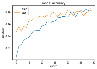
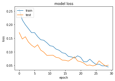
The training curve seems to be DNA structure but tuning our model by adding more layers will come into aid. But I am using this model for now.

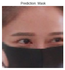
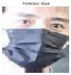
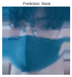
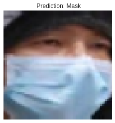
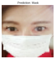
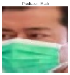
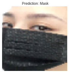
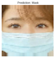
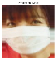
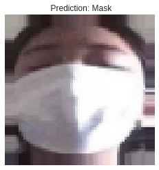
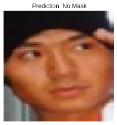
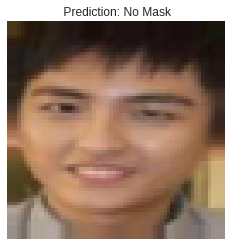
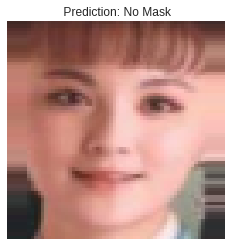
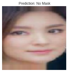
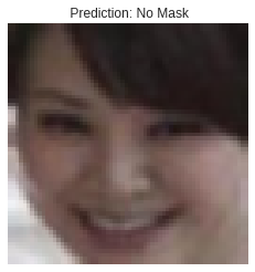
Test It

Lets try to predict some images.

import cv2
plt.style.use('seaborn-whitegrid')
for i in range(15):
    img = validation_generator[0][0][i]
    img = cv2.resize(img, (img_height, img_width))
    img = img.reshape(1, img_height, img_width, 3)
#     lbl = np.argmax(y_test[i])
    prediction = model.predict(img)
#     print(prediction)
    prediction = np.argmax(prediction)
#     print(prediction, lbl)
    classes = ["Mask", "No Mask"]
    title = f" Prediction: {classes[prediction]}"
    plt.imshow(img.reshape(img_height, img_width, 3))
    plt.title(title)
    plt.axis("off")
    plt.show()

png

Save Model

In order to reuse our trained model, we have to save it. Give it a proper name and don’t forget to download it.

# Lets save our model 
from tensorflow.keras.models import model_from_json, load_model

model.save("customCNN64.h5")

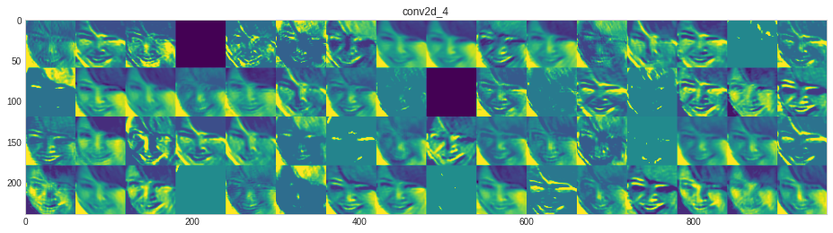
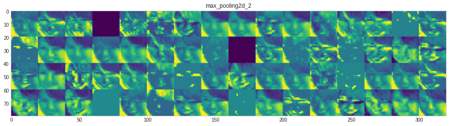
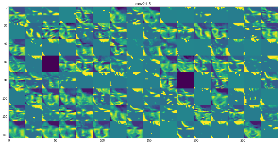
What type of feature each layer has learned?

The code is borrowed from link above the code.

# src https://github.com/gabrielpierobon/cnnshapes/blob/master/README.md
l1, l2=1,-5
layer_outputs = [layer.output for layer in model.layers[l1:l2]] # Extracts the outputs of the top 12 layers
activation_model = Model(inputs=model.input, outputs=layer_outputs)
activations = activation_model.predict(img) # Returns a list of five Numpy arrays: one array per layer activation
# print(img.shape)

layer_names = []
for layer in model.layers[l1:l2]:
    layer_names.append(layer.name) # Names of the layers, so you can have them as part of your plot
    
images_per_row = 16
for layer_name, layer_activation in zip(layer_names, activations): # Displays the feature maps
    n_features = layer_activation.shape[-1] # Number of features in the feature map
    size = layer_activation.shape[1] #The feature map has shape (1, size, size, n_features).
    n_cols = n_features // images_per_row # Tiles the activation channels in this matrix
    if n_cols <1:
      continue
    display_grid = np.zeros((size * n_cols, images_per_row * size))
    for col in range(n_cols): # Tiles each filter into a big horizontal grid
        for row in range(images_per_row):
            channel_image = layer_activation[0,
                                             :, :,
                                             col * images_per_row + row]
            channel_image -= channel_image.mean() # Post-processes the feature to make it visually palatable
            channel_image /= channel_image.std()
            channel_image *= 64
            channel_image += 128
            channel_image = np.clip(channel_image, 0, 255).astype('uint8')
            display_grid[col * size : (col + 1) * size, # Displays the grid
                         row * size : (row + 1) * size] = channel_image
    scale = 1. / size
    #print(size, n_cols, display_grid.shape)
    plt.figure(figsize=(scale * display_grid.shape[1],
                        scale * display_grid.shape[0]))
    plt.title(layer_name)
    plt.grid(False)


    plt.imshow(display_grid, aspect='auto', cmap='viridis')

/usr/local/lib/python3.6/dist-packages/ipykernel_launcher.py:26: RuntimeWarning: invalid value encountered in true_divide

png

Why not read more?

Twitter Facebook LinkedIn

Quassarian Viper