Writing a Linear Regression Class from Scratch Using Python

Contents

• Linear Regression
• Credits
• Linear Regression with only one variable
  • Cost function
  • And hypothesis function is
  • And parameter update rule is
  • Explanation
  • Gradient Descent
• LR with multiple variables
  • How to do Feature Normaliztion?
  • What is the difference between the histograms of normalized data and original?
  • Testing a model
  • But the easiest way of finding parameters is:
• Lets write a class for Linear Regression from scratch.
• Bonus Topic
  • What do you see?
• Finally
  • When to use from scratch or framework?
• Next, we will use Logistic Regression.

Linear Regression

Before there was any ML algorithms, there was a concept and that was regression.

Linear Regression is considered as the process of finding the value or guessing a dependent variable using the number of independent variables. Take for a example:- predicting a price of house using variables like, size of house, age etc.

There are frameworks like scikit-learn which can perform a linear regression on a moment but lets get it from the scratch.

Credits

Credits goes to the author of below repository from where, I have learned the most important concepts of ML and I am using some modified version of codes present there and then I will be using my own version of codes to play with LR from Scratch. This notebook is inspired by the github repo of Tarry Singh and I have referenced most of the codes from that repo. Please leave a star on it.

• Artificial Intelligence Deep Learning Machine Learning Tutorials(Most awesome repository.)
• Dataset is inside machine-learning/Linear Regression/data folder

%matplotlib inline
import numpy as np
import matplotlib.pyplot as plt

Linear Regression with only one variable

Which will be just like the case:- y=mx+c.

# linear regression with one variable
# this file contains comma separated data, first col is profit and second is population
datafile = 'data/ex1data1.txt'
cols = np.loadtxt(datafile, delimiter=',', usecols=(0,1), unpack=True) #Read in comma separated data
#print(cols.shape)
#Form the usual "X" matrix and "y" vector
X = np.transpose(np.array(cols[:-1]))
y = np.transpose(np.array(cols[-1:]))
#print(X.shape)
m = y.size # number of training examples
#Insert the usual column of 1's into the "X" matrix, why?
# to make y = mx + c into np.dot(theta, x), we will add one axis for c.
X = np.insert(X,0,1,axis=1)
print(X.shape, y.shape)

(97, 2) (97, 1)

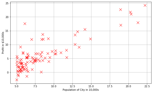
#Plot the data to see what it looks like
plt.figure(figsize=(10,6))
# why X[:, 1]? Every row, but only 1st col
# why y[:, 0]? Every row, but only 0th col
plt.plot(X[:,1], y[:,0],'rx',markersize=10)
plt.grid(True) #Always plot.grid true!
plt.ylabel('Profit in $10,000s')
plt.xlabel('Population of City in 10,000s')

Text(0.5, 0, 'Population of City in 10,000s')

# Lets do gradient Descent
# how many times to run the algorithm?
iterations = 1500
# what is the update step?(learning rate)
alpha = 0.01

Cost function

\begin{equation} J{(\theta)} = \frac{1} {2m} \sum_{i=1}^m (h_\theta (x^{(i)}) - y^{(i)})^2 \end{equation}

And hypothesis function is

\begin{equation} h{_\theta}{(x)} = {\theta}^{T}x = \theta{_0} + \theta{_1} x_1 \end{equation}

And parameter update rule is

\begin{equation} \theta_j = \theta_j - \alpha \frac{1}{m} \sum_{i=1}^m (h_\theta (x^{(i)}) - y^{(i)}) x_j^{(i)} \end{equation}

Where, 𝜃 is parameters of regression.

Explanation

• What is cost function?

  Cost function is a error function which is used to find the error term of a model on a data. On above cost function, ℎ𝜃(𝑥(𝑖)) is the model’s output label. And y(i) is the true label. We find the deviation of the actual label and true label. This is a linear case. We know, the value of (ℎ𝜃(𝑥(𝑖))−𝑦(𝑖)) can be +ve or -ve. And when doing summation, -ve and +ve gets canceled out. So we need to square them and sum it. We will also find mean of. There are varients of cost function for regression. Like:- Mean Squard Error(MSE), Mean Absolute Error(MAE) etc.

• What is hypothesis function?

  In linear regression, simple equation is y = mx + c. The output we want is given by linear combination of x, m, and c. So for us hypothesis function is mx + c. Here m and c are parameters, which are completely independent and we change them to fit our data.

• What is parameter update?

  We start with a simple values(usually, 0s) for parameters and as per finding gradients, we update parameters using the recent gradient value for that parameter. But how? Well, we want to minimize the cost function. So we will find derivative of cost function with respect to parameters. What will be the derivative of 𝐽(𝜃) wrt. 𝜃? And 𝛼 is step for updating gradient. It is often called as learning rate.

• What is 𝑥j(𝑖)?

  It is the input to jth parameter, it can be xj.

def hypothesis_fxn(theta, X): #Linear hypothesis function
    # what is dot product?
    return np.dot(X, theta)

def cost_fxn(theta, X, y): #Cost function
    """
    theta is an n- dimensional vector of initial theta guess
    X is matrix with n- columns and m- rows
    y is a matrix with m- rows and 1 column
    """
    
    # see the cost function
    # find hypothesis
    h = hypothesis_fxn(theta, X)
    
    # find actual deviation
    d = h - y 
    
    # constant 1/2m
    c = 1/(2 * m)
    
    # finally, sum the square of gradients 
    delta = c * np.sum(d ** 2)   
    #print(delta, sum(c*d**2))
    return delta

#Test that running computeCost with 0's as theta returns 32.07:

initial_theta = np.zeros((X.shape[1],1)) #(theta is a vector with n rows and 1 columns (if X has n features) )
print(cost_fxn(initial_theta,X,y))

32.072733877455676

Gradient Descent

The overall concept of Gradient Descent is that,

“Remember you are at the peak of mountain, your goal is to reach the bottom of mountain. Where will you move? Downwards but slowly. We update our parameter towards the direction of gradient using gradient.”

\begin{equation} \delta(\theta) = - \frac{d(J(\theta))}{d(\theta)} \end{equation}

The -ve sign indicates that we are decreasing the value.

# gradient descent
def gradient_descent(X, theta=np.zeros(2)):
    """
    theta is an n- dimensional vector of initial theta guess
    X is matrix with n- columns and m- rows
    """
    costs = [] #Used to plot cost as function of iteration
    theta_history = [] #Used to visualize the minimization path later on
    for i in range(iterations):
        temp_theta = theta
        c = cost_fxn(theta, X, y)
        costs.append(c)
        # Fixed line
        theta_history.append(list(theta[:,0]))
        
        #Simultaneously updating theta values
        for j in range(len(temp_theta)):
            # see the update rule above for explanation of this code
            # 𝜃𝑗=𝜃𝑗−𝛼/𝑚 * ∑𝑖=1𝑚(ℎ𝜃(𝑥(𝑖))−𝑦(𝑖))
            #print((hypothesis_fxn(initial_theta, X) - y).shape, np.array(X[:,j]).shape)
            temp_theta[j] = theta[j] - (alpha / m) * np.sum((hypothesis_fxn(initial_theta, X) - y)*np.array(X[:,j]).reshape(m, 1))
        theta = temp_theta
        #print("it", initial_theta, theta)
    return theta, theta_history, costs

#Actually run gradient descent to get the best-fit theta values
initial_theta = np.zeros((X.shape[1],1))
# print(initial_theta)
theta, thetahistory, jvec = gradient_descent(X, initial_theta)
jvec = np.array(jvec).reshape(-1, 1)
# print(initial_theta)
#print(jvec)
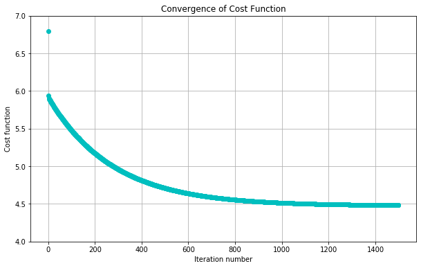
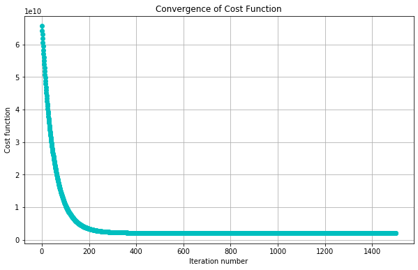
#Plot the convergence of the cost function
def plotConvergence(jvec):
    plt.figure(figsize=(10,6))
    plt.plot(range(len(jvec)),jvec,'co')
    plt.grid(True)
    plt.title("Convergence of Cost Function")
    plt.xlabel("Iteration number")
    plt.ylabel("Cost function")
    dummy = plt.xlim([-0.05*iterations,1.05*iterations])
    #dummy = plt.ylim([4,8])


plotConvergence(jvec)
dummy = plt.ylim([4,7])

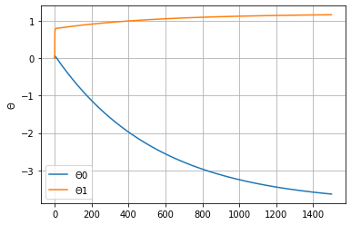
thetas = np.array(thetahistory)
plt.plot(thetas)
plt.grid(True)
plt.legend([r"$\Theta0$", r"$\Theta1$"])
plt.ylabel(r"$\Theta$")

Text(0, 0.5, '$\\Theta$')

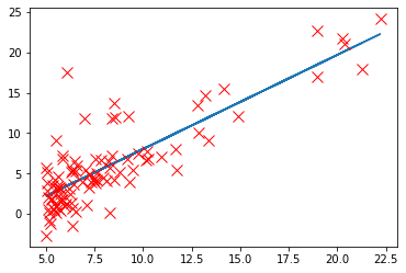
# we h've found best thetas for our problem now is the time to predict
def prediction(theta, x):
    return theta[0] + theta[1] * x

pred = prediction(theta, X[:, 1]) 
# plt.plot(X[:,1],myfit(X[:,1]),'c-',label = 'Hypothesis: h(x) = %0.2f + %0.2fx'%(theta[0],theta[1]))
plt.plot(X[:, 1], pred)
plt.plot(X[:,1],y[:,0],'rx',markersize=10,label='Training Data')

[<matplotlib.lines.Line2D at 0x274da862c48>]

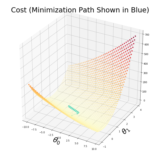
#Import necessary matplotlib tools for 3d plots
from mpl_toolkits.mplot3d import axes3d, Axes3D
from matplotlib import cm
import itertools

# create a figure where we want to draw 
fig = plt.figure(figsize=(12,12))

# prepare axis for 3d
ax = fig.gca(projection='3d')

# prepare xvals
xvals = np.arange(-10,10,.5)

# prepare y vals
yvals = np.arange(-1,4,.1)
myxs, myys, myzs = [], [], []

# now our z should be the loss value
for xv in xvals:
    for yv in yvals:
        myxs.append(xv)
        myys.append(yv)
        myzs.append(cost_fxn(np.array([[xv], [yv]]),X,y))

# scatter the values
scat = ax.scatter(myxs,myys,myzs,c=np.abs(myzs),cmap=plt.get_cmap('YlOrRd'))

plt.xlabel(r'$\theta_0$',fontsize=30)
plt.ylabel(r'$\theta_1$',fontsize=30)
plt.title('Cost (Minimization Path Shown in Blue)',fontsize=30)
plt.plot([x[0] for x in thetahistory],[x[1] for x in thetahistory],jvec.reshape(len(jvec)),'co-')
plt.show()

LR with multiple variables

While using multiple parameters, we might strike different problems of convergence. One way of avoiding is by doing Normalization. The way of normalizing feature is known as Feature Normalization. The dataset we will be using here consists of 3 columns.

• Size of the house (in square feet)
• Number of bedrooms
• Price of the house.

How to do Feature Normaliztion?

• Subtract the mean value of each feature from the dataset.
• After subtracting the mean, additionally scale (divide) the feature values by their respective “standard deviations”.

Implementation Note: When normalizing the features, it is important to store the values used for normalization - the mean value and the standard deviation used for the computations. After learning the parameters from the model, we often want to predict the prices of houses we have not seen before. Given a new x value (living room area and number of bedrooms), we must first normalize x using the mean and standard deviation that we had previously computed from the training set.

In the multivariate case, the cost function can also be written in the following vectorized form: \begin{equation} J{(\theta)} = \frac{1} {2m} (X\theta - \vec y)^T (X\theta - \vec y) \end{equation}

Where, \begin{equation} X = \begin{pmatrix} \cdots & (x^{(1)})^T & \cdots
\cdots & (x^{(2)})^T & \cdots
\vdots & \vdots & \vdots
\cdots & (x^{(m)})^T & \cdots
\end{pmatrix}, \vec y = \begin{pmatrix} (y^{(1)})^T
(y^{(2)})^T
\vdots
(y^{(m)})^T
\end{pmatrix} \end{equation}

datafile = 'data/ex1data2.txt'
#Read into the data file
cols = np.loadtxt(datafile,delimiter=',',usecols=(0,1,2),unpack=True) #Read in comma separated data
#Form the usual "X" matrix and "y" vector
X = np.transpose(np.array(cols[:-1]))
y = np.transpose(np.array(cols[-1:]))
m = y.size # number of training examples
#Insert the usual column of 1's into the "X" matrix
X = np.insert(X,0,1,axis=1)

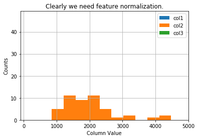
Visualise our data, which is not normalized right now.

#Quick visualize data
plt.grid(True)
plt.xlim([-100,5000])
dummy = plt.hist(X[:,0],label = 'col1')
dummy = plt.hist(X[:,1],label = 'col2')
dummy = plt.hist(X[:,2],label = 'col3')
plt.title('Clearly we need feature normalization.')
plt.xlabel('Column Value')
plt.ylabel('Counts')
dummy = plt.legend()

# We have 3 columns and col3 is for prediction of houses
# we need to find mean, std of all the columns
means, stds = [], []
normalized_x = X.copy()
# since we need to work with only the column we will iterate over shape[1]
for col in range(normalized_x.shape[1]):
    means.append(normalized_x[:, col].mean())
    stds.append(normalized_x[:, col].std())
    if not col: continue
    normalized_x[:, col] = (normalized_x[:, col] - means[-1])/stds[-1]

#Quick visualize the feature-normalized data
plt.grid(True)
plt.xlim([-5,5])
dummy = plt.hist(normalized_x[:,0],label = 'col1')
dummy = plt.hist(normalized_x[:,1],label = 'col2')
dummy = plt.hist(normalized_x[:,2],label = 'col3')
plt.title('Feature Normalization Accomplished')
plt.xlabel('Column Value')
plt.ylabel('Counts')
dummy = plt.legend()

What is the difference between the histograms of normalized data and original?

Well, normalized data tends to be more spreaded.

# how many parameters will there be?
# for n features, there will be n + 1
# since our input data have new axis already added for the bias term, we will initialize parameters only n
initial_theta = np.zeros((normalized_x.shape[1],1))

theta, thetahistory, jvec = gradient_descent(normalized_x, initial_theta)

#Plot convergence of cost function:
plotConvergence(jvec)

# lets view our thetas, 
theta

array([[340412.56301439],
       [109371.67272252],
       [ -6502.3992545 ]])

Testing a model

# lets test our model if it is working fine.
# we created a model by normalizing features, so we have to convert test data into same as train data
print( "Check of result: What is price of house with 1650 square feet and 3 bedrooms?")
test = np.array([1650, 3])

# scale test data
test_scaled = [(test[x] - means[x+1]) / stds[x+1] for x in range(len(test))]
test_scaled.insert(0, 1) # remember, we have inserted one axis on our X i.e we added a term for bias.
print("Answer: $%0.2f" % float(hypothesis_fxn(theta, test_scaled)))

Check of result: What is price of house with 1650 square feet and 3 bedrooms?
Answer: $293098.15

But the easiest way of finding parameters is:

\begin{equation} \theta = (X^T X)^{-1} X^T \vec y \end{equation}

But here, every X will be non normalized.

thetas = np.dot(np.dot(np.linalg.inv(np.dot(X.T, X)), X.T), y)

print("Answer: $%0.2f" % float(hypothesis_fxn(thetas, [1, 1650, 3])))

Answer: $293081.46

Lets write a class for Linear Regression from scratch.

I have used some of codes above to write a class of LR.

import numpy as np
import matplotlib.pyplot as plt

class LinearRegression:
    """
        A simple class to perform a task of Linear Regression.
        
        Steps
        -----
        * Find the hypothesis using y = mX + c, where X is as input vector.
        * Find the cost value.
        * Use gradient descent to update each parameters.
    """
    def __init__(self):
        """
            This method doesnot take any initial attributes. You will tune the attributes later using methods.
        """
        # instantiate train data and label
        self.X = None 
        self.y = None
        # to store all costs, initially cost is infinity
        self.costs = [np.inf]
        
        # m is for len(X)
        self.m = None
        
        # learning rate
        self.alpha = None
        
        # our all parameters(from each iterations), m, c in y = mx + c
        self.all_parameters = []
    
    def hypothesis(self, x):
        """
            A method to perform linear operation(mx + c) and return.
            
            Formula:
            --------
            \begin{equation}
            h{_\theta}{(x)} = {\theta}^{T}x = \theta{_0} + \theta{_1} x_1 
            \end{equation}

        """
        # y = XM, where X is of shape (M, N) and M of (N, 1)
        h = np.dot(x, self.parameters)
        return h
    
    def cost(self, yp, yt):
        """
            yp: Predicted y.
            yt: True y.

            Formula:
            -------
            \begin{equation}
            J{(\theta)} = \frac{1} {2m} \sum_{i=1}^m (h_\theta (x^{(i)}) - y^{(i)})^2
            \end{equation}

        """
        # find actual deviation
        d = yp - yt 
        # constant 1/2m
        c = 1/(2 * self.m)
        # finally, sum the square of gradients 
        delta = c * np.sum(d ** 2)   
        return delta
    
    def gradient_descent(self):
        """
            A method to perform parameter update based on gradient descent algorithm.
            
            Rule:
            -----
            \begin{equation}
            \theta_j = \theta_j - \alpha \frac{1}{m} \sum_{i=1}^m (h_\theta (x^{(i)}) - y^{(i)}) x_j^{(i)}
            \end{equation}

        """
        temp_theta = self.parameters
        # for each theta
        for j in range(len(temp_theta)):
            grad = np.sum((self.hypothesis(self.X) - self.y)*np.array(self.X[:,j]).reshape(self.m, 1))
            temp_theta[j] = self.parameters[j] - (self.alpha / self.m) * grad
        self.parameters = temp_theta
        self.all_parameters.append(temp_theta.flatten())
        
    def predict(self, X):
        """
            A method to return prediction. Perform preprocessing if model was trained preprocessed data.

            Preprocessing:
            -------------
            X = (X - X.mean()) / X.std()
        """
        if self.preprocessed != True:
            X = np.insert(X, 0, 1, axis=1)
            X = self.normalize(X)
        return self.hypothesis(X)
    
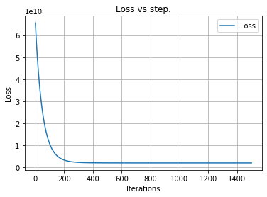
    def visualize(self, thing="cost"):
        """
            Visualise the plots.
            Available thing:
            ----------
            i. cost: Cost value vs iteration
            ii. param: Parameters vs iteration
            iii. all: cost and param vs iteration
        """
        legend = ["Loss"]
        if thing == "cost" or thing == "all":
            plt.title("Loss vs step.")
            plt.grid(True)
            plt.plot(self.costs)
            plt.xlabel("Iterations")
            plt.ylabel("Loss")
            plt.legend(legend)
    
    #def visualize_parameters(self):
        if thing == "param" or thing == "all":
            plt.title("Parameter on each step.")
            plt.grid(True)
            plt.plot(self.all_parameters)
            plt.xlabel("Iterations")
            plt.ylabel("Parameters")
            l = [fr"$\Theta{i}$" for i in range(len(self.parameters))]
            if thing == "all":
                l.insert(0, legend[0])
                legend = l
            else:
                legend = l
            plt.legend(legend)
        
    def normalize(self, X):
        """
            X: Input training data.
            Returns: normalized x.
            
            Normalization:
            --------------
            X = (X - X.mean()) / X.std()
        
        """
        
        means, stds = [], []
        normalized_x = X.copy()
        # since we need to work with only the column we will iterate over shape[1]
        for col in range(normalized_x.shape[1]):
            means.append(normalized_x[:, col].mean())
            stds.append(normalized_x[:, col].std())
            if not col: continue
            normalized_x[:, col] = (normalized_x[:, col] - means[-1])/stds[-1]
        # store the means and stds. We need them on future.
        self.means = means
        self.stds = stds
        return normalized_x

    def fit(self, X, y, error_threshold = 0.001, preprocessed = True, alpha=0.01, show_every=100, iterations=1500):
        """
            X: input train (m X n),  if is not normalized and added axis for bias, use preprocessed=False.
            y: train label (n X 1)
            error_threshold: How much error is tolerable?
            preprocessed: does train data has added axis for bias and normalized?
            alpha: learning rate(update step)
            show_every: how often to show cost?
            iterations: how many steps to run weight update(gradient descent)?
        """
        
        self.preprocessed = preprocessed
        # if data already have bias added and normalized, leave it.
        if preprocessed!=True:
            X = np.insert(X, 0, 1, axis=1)
            X = self.normalize(X)
        self.X = X
        self.y = y
        self.alpha = alpha
        
        # how many of training examples are there?
        self.m = len(X)
        
        # how many of parameters?
        # initialize it to 0, shape must be (num. features + 1, 1)
        # X here is normalized i.e it already have axis for bias
        self.parameters = np.zeros((X.shape[1], 1))
        costs = [np.inf] #Used to plot cost as function of iteration
        i = 0
        
        # if our update is not done for iterations and error is pretty high, 
        while (iterations>i and costs[-1]>error_threshold):
            # find the cost value
            cost_value = self.cost(self.hypothesis(self.X), self.y)
            costs.append(cost_value)
            # perform gradient descent and update param
            self.gradient_descent() 
            if i % show_every == 0:
                print(f"Step: {i} Cost: {round(cost_value, 4)}.")
            
            i+=1
        self.costs = costs

lr = LinearRegression()

lr.fit(normalized_x[:, :], y, iterations=1500)

Step: 0 Cost: 65591548106.4574.
Step: 100 Cost: 10595100091.847.
Step: 200 Cost: 3342249838.3436.
Step: 300 Cost: 2286559555.6221.
Step: 400 Cost: 2104727177.9675.
Step: 500 Cost: 2063437958.1946.
Step: 600 Cost: 2050905508.0485.
Step: 700 Cost: 2046335257.1982.
Step: 800 Cost: 2044529088.4146.
Step: 900 Cost: 2043794129.3507.
Step: 1000 Cost: 2043492101.0415.
Step: 1100 Cost: 2043367581.1412.
Step: 1200 Cost: 2043316190.0075.
Step: 1300 Cost: 2043294972.882.
Step: 1400 Cost: 2043286212.2944.

# lets check our parameters
lr.parameters

array([[340412.56301439],
       [109371.67272252],
       [ -6502.3992545 ]])

# lets visualize our loss per steps
lr.visualize()
plt.show()

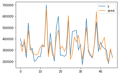
# lets visualize our prediction with real label
plt.plot(y, label="y")
plt.plot(lr.predict(normalized_x), label="pred")
plt.legend()

<matplotlib.legend.Legend at 0x274dab56f48>

Bonus Topic

Check our model with sklearn’s LinearRegressionto work with boston_housing dataset.

This dataset is an example of linear regression dataset where our attempt will be to train a model to find a best fit of parameters for the regression problems. There are 13 columns and each represents distinct features. We will compare our model’s and Sklearn’s model.

# import the linear regression class and boston dataset
from sklearn.linear_model import LinearRegression
from sklearn.datasets import load_boston

# load dataset, it will be on dictionary
boston = load_boston()
bX = boston["data"]
by = boston["target"].reshape(-1, 1)

# train our model 
lr.fit(bX, by, preprocessed=False, show_every=5000, iterations=15000)

Step: 0 Cost: 296.0735.
Step: 5000 Cost: 10.948.
Step: 10000 Cost: 10.9474.

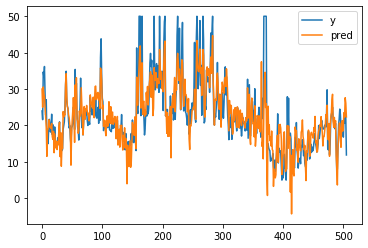
# get prediction
p1 = lr.predict(bX)

# visualise the predicted vs real labels
plt.plot(by[:, 0], label="y")
plt.plot(p1, label="pred")
plt.legend()

<matplotlib.legend.Legend at 0x274e55eaa08>

# use sklearn's class
m = LinearRegression()
m.fit(bX, by)

LinearRegression(copy_X=True, fit_intercept=True, n_jobs=None, normalize=False)

# get prediction
p2 = m.predict(bX)
plt.plot(by[:, 0], label="y")
plt.plot(p2, label="pred")
plt.legend()

<matplotlib.legend.Legend at 0x274e36c8188>

What do you see?

You should not expect our model to compete with sklearn, but it is worth trying to do it from scratch.

# lets visualize our prediction with real label
plt.plot(by[:, 0], label="y")
plt.plot(p1, label="our model")
plt.plot(p2, label="sklearn")
plt.legend()

<matplotlib.legend.Legend at 0x274e7688a08>

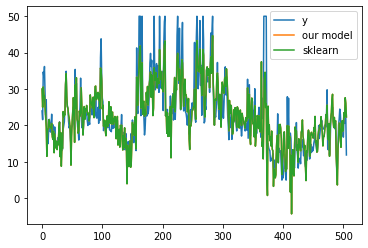
## How about checking mse?
diff = np.mean((p1 - p2)**2)
diff

3.4921935541453176e-09

Finally

On above block, we can clearly see that mse is very low between sklearn’s output and our model’s output. Which means than we did really great.

When to use from scratch or framework?

• When we have enough time to cover mathematics and of course on teaching.
• When we have to work on production level, we should use framework.

Next, we will use Logistic Regression.