World Cup Tweet Sentiment Analysis in Python with Tweepy and TextBlob

The World Cup is one of the biggest sports events in the world, and social media becomes very active during the tournament. Fans support their teams, react to matches, discuss players, and sometimes argue with people who support the opposite side.

This makes World Cup tweets a useful dataset for a small sentiment analysis project in Python. In this post, I will collect World Cup related tweets, clean the tweet text, classify each tweet as positive, neutral, or negative, and visualize the results.

This tutorial uses:

• Tweepy to collect tweets
• pandas to work with the dataset
• TextBlob to calculate sentiment
• matplotlib to create visualizations

The goal is not to build a perfect sentiment model. The goal is to create a simple end-to-end workflow for World Cup tweet sentiment analysis in Python.

Note: This post uses the Twitter API workflow that was available when the original experiment was written. If you are running this today, check the current Twitter/X API access rules and Tweepy documentation before collecting data.

Project Overview

The sentiment analysis workflow has five main steps:

1. collect tweets related to the World Cup
2. save tweets into a CSV file
3. clean the tweet text
4. calculate sentiment with TextBlob
5. visualize sentiment distribution and tweet activity

The keywords used for collecting tweets are:

kwds = [
    "worldcup",
    "world cup",
    "wcup",
    "football",
    "qatar worldcup prediction"
]

Getting World Cup Tweet Data

The first step is to collect tweets related to the World Cup. I used Tweepy for this.

I have a separate walkthrough on scraping tweets with Tweepy here:

• Tweet Scraping Using Tweepy

You can install Tweepy with:

pip install tweepy

In the original notebook, I installed the development version from GitHub:

!pip install git+https://github.com/tweepy/tweepy.git

For most cases, the normal pip install tweepy command is easier.

Set Twitter API Keys

To use the Twitter API, you need API credentials.

api_key = "api_key_here"
api_secret = "api_secret_here"
bearer = "bearer_here"
access_token = "access_token_here"
access_token_secret = "access_token_secret_here"

Do not publish real API keys in your blog, GitHub repository, or notebook. Use environment variables or a .env file for real projects.

Connect to the Twitter API with Tweepy

Now, we can create a Tweepy API connection.

import tweepy as tw

auth = tw.OAuthHandler(api_key, api_secret)
auth.set_access_token(access_token, access_token_secret)

api = tw.API(auth, wait_on_rate_limit=True)

If there is no error, the connection is working.

Function to Collect Related Tweets

The function below searches tweets for a list of keywords and writes the results to a CSV file.

import csv
import os
import time

import pandas as pd


def get_related_tweets(key_words, language="en", max_tweets=5000, max_items=500):
    """Collect tweets related to given keywords and save them into a CSV file.

    Parameters
    ----------
    key_words : list[str]
        List of search keywords.
    language : str
        Tweet language filter.
    max_tweets : int
        Maximum number of tweets to collect.
    max_items : int
        Maximum number of tweets to request for each keyword.

    Returns
    -------
    pandas.DataFrame
        DataFrame containing collected tweets.
    """
    file_name = language + str(time.time()) + ".csv"
    print(f"Filename: {file_name}")

    count = 0

    for key_word in key_words:
        print(f"Current keyword: {key_word}")

        for tweet in tw.Cursor(
            api.search_tweets,
            q=key_word,
            count=max_items
        ).items(max_items):

            if tweet.lang != language:
                continue

            try:
                status = api.get_status(tweet.id, tweet_mode="extended")

                try:
                    tweet_text = status.retweeted_status.full_text
                except AttributeError:
                    tweet_text = status.full_text

                row = {
                    "id": tweet.id,
                    "tweet_created_at": tweet.created_at,
                    "text": tweet_text,
                    "user": tweet.user.screen_name,
                    "bio": tweet.user.description,
                    "location": tweet.user.location,
                    "hashtags": tweet.entities["hashtags"],
                    "user_mentions": len(tweet.entities["user_mentions"]),
                    "in_reply": tweet.in_reply_to_status_id,
                    "protected": tweet.user.protected,
                    "followers_count": tweet.user.followers_count,
                    "friends_count": tweet.user.friends_count,
                    "listed_count": tweet.user.listed_count,
                    "created_at": tweet.user.created_at,
                    "favourites_count": tweet.user.favourites_count,
                    "geo_enabled": tweet.user.geo_enabled,
                    "verified": tweet.user.verified,
                    "statuses_count": tweet.user.statuses_count,
                    "coordinates": tweet.coordinates,
                    "is_quote_status": tweet.is_quote_status,
                    "retweet_count": tweet.retweet_count,
                    "retweeted": tweet.retweeted,
                    "lang": tweet.lang,
                    "source": tweet.source,
                    "place": tweet.place,
                    "kwd": key_word,
                }

                file_exists = os.path.isfile(file_name)

                with open(file_name, "a", encoding="utf-8", newline="") as csvfile:
                    writer = csv.DictWriter(csvfile, fieldnames=list(row.keys()))

                    if not file_exists:
                        writer.writeheader()

                    writer.writerow(row)

                count += 1

                if count >= max_tweets:
                    break

            except Exception as error:
                print(f"Skipping tweet because of error: {error}")

    return pd.read_csv(
        file_name,
        parse_dates=["tweet_created_at", "created_at"]
    )

Now, run the function with the World Cup keywords.

kwds = [
    "worldcup",
    "world cup",
    "wcup",
    "football",
    "qatar worldcup prediction"
]

df = get_related_tweets(kwds)

The collected CSV file in this experiment contained 1849 tweets and 26 columns.

Read the Saved CSV File

After collecting tweets, we can read the CSV file directly.

df = pd.read_csv("en1670670038.8448372.csv")
df.head()

The important columns for this sentiment analysis are:

df[["tweet_created_at", "text", "user", "source", "kwd"]].head()

The text column contains the tweet content, and tweet_created_at tells us when the tweet was created.

Clean Tweet Text

Raw tweets are noisy. They often contain:

• mentions such as @username
• hashtags
• links
• emojis
• punctuation
• line breaks
• numbers

Before sentiment analysis, we should clean the text.

import re
import string


def remove_noise(tweet):
    """Remove common noise from tweet text."""
    tweet = str(tweet)

    # Remove URLs
    tweet = re.sub(r"http\S+|www\S+|https\S+", " ", tweet)

    # Remove mentions
    tweet = re.sub(r"@\w+", " ", tweet)

    # Remove hashtag symbol but keep the word
    tweet = re.sub(r"#", "", tweet)

    # Remove punctuation
    tweet = re.sub(f"[{re.escape(string.punctuation)}]", " ", tweet)

    # Remove numbers
    tweet = re.sub(r"\w*\d\w*", " ", tweet)

    # Remove extra spaces
    tweet = " ".join(tweet.split())

    return tweet

Now, apply the cleaning function to the tweet text.

df["clean_text"] = df["text"].apply(remove_noise)

df[["text", "clean_text"]].head()

The cleaned text is not perfect, but it is good enough for a simple TextBlob sentiment analysis.

Calculate Tweet Sentiment with TextBlob

For sentiment classification, I used TextBlob.

You can install it with:

pip install textblob

Then import it:

from textblob import TextBlob

The function below classifies a tweet as positive, neutral, or negative based on polarity.

def get_sentiment(tweet):
    """Return positive, neutral, or negative sentiment for a tweet."""
    analysis = TextBlob(tweet)

    if analysis.sentiment.polarity > 0:
        return "positive"

    if analysis.sentiment.polarity == 0:
        return "neutral"

    return "negative"

Now, apply the function to the cleaned tweets.

df["sentiment"] = df["clean_text"].apply(get_sentiment)

df[["clean_text", "sentiment"]].head()

TextBlob gives a polarity score. A positive polarity means the text is positive, zero means neutral, and a negative polarity means the text is negative.

Plot Sentiment Distribution

Now, let’s plot the sentiment distribution.

import matplotlib.pyplot as plt

df["sentiment"].value_counts().plot(
    kind="pie",
    figsize=(15, 10),
    autopct="%1.1f%%"
)

plt.title("World Cup Tweet Sentiment Distribution")
plt.ylabel("")
plt.show()

Most tweets in this dataset seem to be neutral. This is expected because many tweets may contain news, predictions, links, or simple match updates instead of clear emotional language.

Tweets Per User

We can also check how often each user appears in the dataset.

df["user"].value_counts().hist()

plt.title("Tweets Per User")
plt.xlabel("Number of tweets")
plt.ylabel("Number of users")
plt.show()

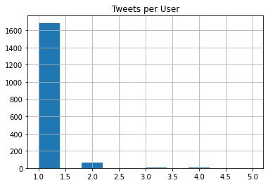
It seems that only a few users posted more than one tweet in this collected dataset.

Tweet Source Distribution

Tweets can come from different sources such as Android, iPhone, web, or social media management tools.

There are many sources in the dataset, so I only plot the top three.

top_sources = df["source"].value_counts().head(3).index

df[df["source"].isin(top_sources)]["source"].hist()

plt.title("Top Tweet Sources")
plt.xlabel("Source")
plt.ylabel("Number of tweets")
plt.show()

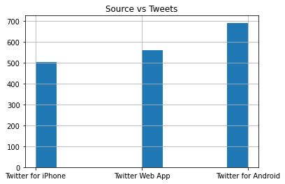
In this dataset, Android users appear very often among the top tweet sources.

Tweets Per Day

The tweet_created_at column can be used to analyze when tweets were posted.

df["date"] = pd.to_datetime(df["tweet_created_at"]).dt.date

df["date"].value_counts().sort_index().plot(
    kind="bar",
    figsize=(15, 10)
)

plt.title("World Cup Tweets Per Day")
plt.xlabel("Date")
plt.ylabel("Number of tweets")
plt.show()

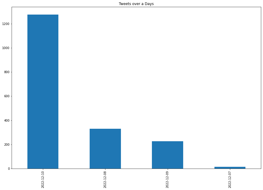
The latest date in this collected sample has the most tweets. This may change if we collect more tweets or collect tweets during a different match period.

Tweets by Hour

We can also check the hour when tweets were posted.

pd.to_datetime(df["tweet_created_at"]).dt.hour.value_counts().sort_index().plot(
    kind="bar",
    figsize=(15, 10)
)

plt.title("Distribution of World Cup Tweets by Hour")
plt.xlabel("Hour")
plt.ylabel("Number of tweets")
plt.show()

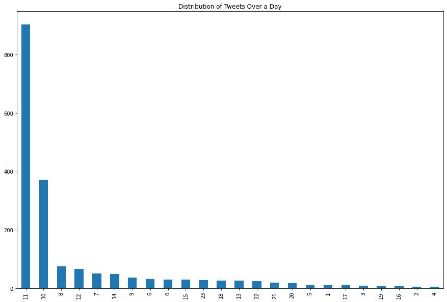
In this dataset, most tweets were posted around 11 AM.

Sentiment by Hour

Next, let’s check the sentiment distribution by hour.

df["hour"] = pd.to_datetime(df["tweet_created_at"]).dt.hour

df[["hour", "sentiment"]].value_counts().plot(
    kind="bar",
    figsize=(15, 10)
)

plt.title("World Cup Tweet Sentiment by Hour")
plt.xlabel("Hour and sentiment")
plt.ylabel("Number of tweets")
plt.show()

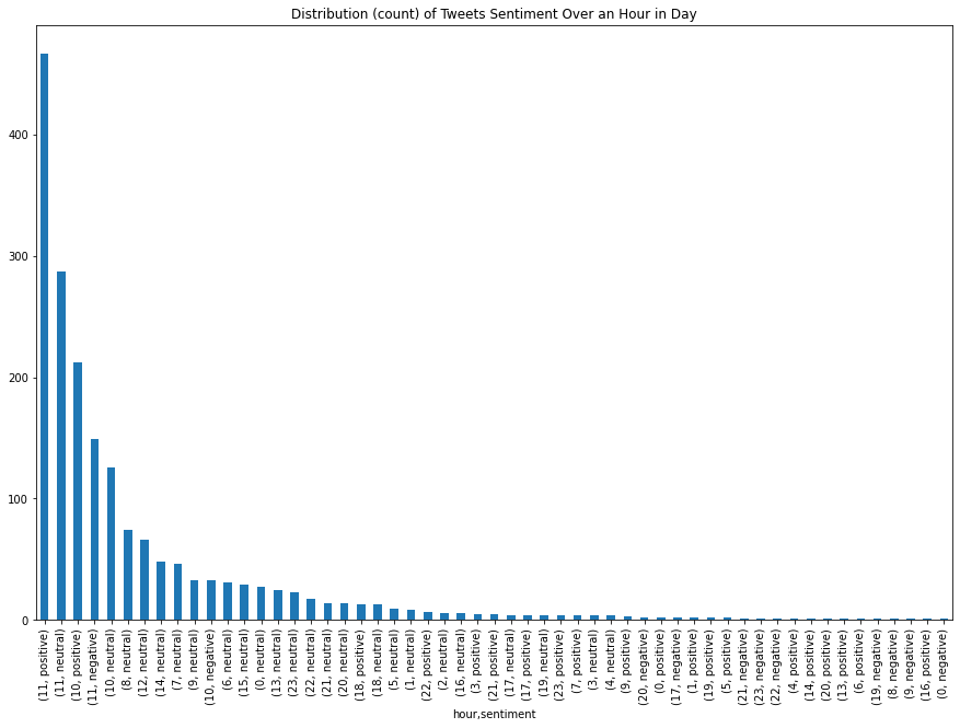
The count plot is useful, but it can be hard to compare sentiment across hours.

So, we can also plot normalized values.

df[["hour", "sentiment"]].value_counts(normalize=True).plot(
    kind="bar",
    figsize=(15, 10)
)

plt.title("World Cup Tweet Sentiment Ratio by Hour")
plt.xlabel("Hour and sentiment")
plt.ylabel("Ratio")
plt.show()

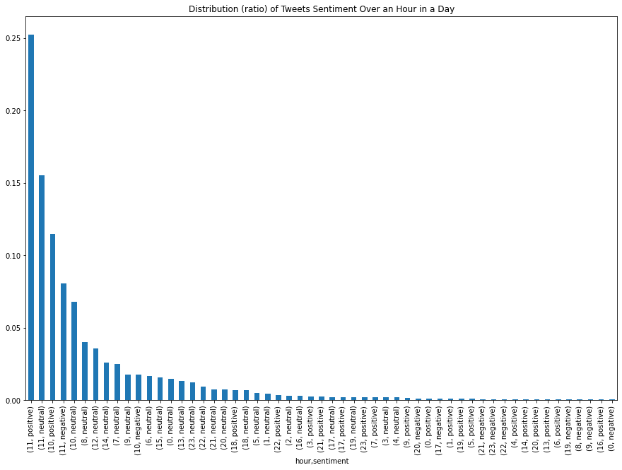
This plot gives a rough idea of how sentiment is distributed across different hours, but the dataset is small, so we should not make strong conclusions from it.

WordCloud of World Cup Tweets

A good next step is to create a WordCloud from the tweet text. I wrote a separate post for that:

• WordCloud in Python: Text Analysis and Twitter Data Visualization

A WordCloud can help us quickly see which words appear most often in the World Cup tweet dataset.

Limitations of This Sentiment Analysis

This is a simple sentiment analysis project, so it has some limitations:

• TextBlob may not understand sarcasm.
• Short tweets can be hard to classify.
• Sports tweets often include slang, emojis, team names, and abbreviations.
• The dataset is small and collected from a limited keyword list.
• The sentiment result depends heavily on text cleaning.
• Retweets or repeated text can affect the distribution.

For a more serious project, we could use a larger dataset, remove duplicates, compare multiple sentiment models, or fine-tune a transformer-based model.

Further Analysis Ideas

This dataset can be used to answer more questions, such as:

• What is the sentiment distribution based on tweet source?
• Which hours have the highest number of negative tweets?
• Which days have the most positive tweets?
• Do users who tweet many times show different sentiment patterns?
• Which keywords produce more positive or negative tweets?
• Is sentiment different before and after important matches?
• What are the most common words in positive and negative tweets?

Final Thoughts

In this post, I showed a simple workflow for World Cup tweet sentiment analysis in Python. We collected tweets using Tweepy, cleaned the tweet text, classified sentiment using TextBlob, and visualized the results with pandas and matplotlib.

The result showed that many tweets were neutral in this dataset. This makes sense because World Cup tweets often include predictions, match updates, links, and general discussion.

This project is a good starting point for learning social media analysis, NLP, and sentiment analysis with Python.