
Writing a Logistic Regression Class from Scratch
Contents
Logistic Regression
Logistic Regression is not exactly a regression but it performs a classification. As the name suggests, it uses the logistic function.
This notebook is inspired by the github repo of Tarry Singh and I have referenced most of the codes from that repo. Please leave a star on it.
- Artificial Intelligence Deep Learning Machine Learning Tutorials(Most awesome repository.)
- Dataset is inside
machine-learning/Logistic Regression/datafolder
And the dataset we are using here can be found inside same repository .
# import dependencies
import numpy as np
import matplotlib.pyplot as plt
import pandas as pd
%matplotlib inline
The problem we are tackling:-
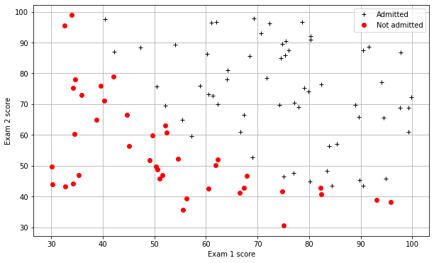
In this part of the tutorial, we will build a logistic regression model to predict whether a student gets admitted into a university. Suppose that you are the administrator of a university department and you want to determine each applicant’s chance of admission based on their results on two exams. You have historical data from previous applicants that you can use as a training set for logistic regression. For each training example, you have the applicant’s scores on two exams and the admissions decision. Your task is to build a classification model that estimates an applicant’s probability of admission based the scores from those two exams.
Prepare Data
# read data file
datafile = 'data/ex2data1.txt'
#!head $datafile
cols = np.loadtxt(datafile,delimiter=',',usecols=(0,1,2),unpack=True) #Read in comma separated data
##Form the usual "X" matrix and "y" vector
X = np.transpose(np.array(cols[:-1]))
y = np.transpose(np.array(cols[-1:]))
m = y.size # number of training examples
##Insert the usual column of 1's into the "X" matrix, why?
X = np.insert(X,0,1,axis=1)
Visualize Data
# Divide the sample into two: ones with positive classification, one with null classification
# it is a part of list comprehension
# loop through every rows and if the label for that row is 1 add it to pos else add it to neg
pos = np.array([X[i] for i in range(X.shape[0]) if y[i] == 1])
neg = np.array([X[i] for i in range(X.shape[0]) if y[i] == 0])
def plotData():
    plt.figure(figsize=(10,6))
    plt.plot(pos[:,1],pos[:,2],'k+',label='Admitted')
    plt.plot(neg[:,1],neg[:,2],'ro',label='Not admitted')
    plt.xlabel('Exam 1 score')
    plt.ylabel('Exam 2 score')
    plt.legend()
    plt.grid(True)

plotData()
Implementation
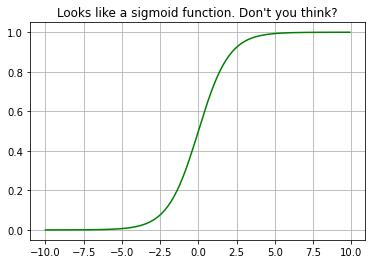
Logistic regression is based on the logistic function. Look the beauty of the function, it takes input from range of (-infinity, infinity) and the output will be on the range (0, 1). The graph of this function is like the S hence called sigmoid.
\begin{equation}
\sigma(x) = \frac{1}{1 + e^{(-x)}}
\end{equation}
from scipy.special import expit #Vectorized sigmoid function
#Quick check that expit is what I think it is
myx = np.arange(-10,10,.1)
plt.plot(myx,expit(myx), 'g')
plt.title("Looks like a sigmoid function. Don't you think?")
plt.grid(True)

def expit(x):
    return 1 / (1+np.exp(-x))
#Quick check that expit is what I think it is
myx = np.arange(-10,10,.1)
plt.plot(myx,expit(myx), 'g')
plt.title("Looks like a sigmoid function. Don't you think?")
plt.grid(True)
Hypothesis function
\begin{equation} h_\theta(x) = \sigma(\theta^Tx) \end{equation}
Cost function
We are using crossentropy here. The beauty of this cost function is that, due to being log loss, the true negative and false positive values are punished more. In other words, if the prediction is not 100% sure, then model is penalized always.

Parameter Update
The derivative of cost function with respect to theta will be: \begin{equation} \theta_j = \theta_j - \alpha \frac{1}{m} \sum_{i=1}^m (h_\theta (x^{(i)}) - y^{(i)}) x_j^{(i)} \end{equation}
If we use square loss and its derivative for the parameter update. \begin{equation} \theta_j = \theta_j - \alpha \frac{1}{m} \sum_{i=1}^m (h_\theta (x^{(i)}) - y^{(i)})* h_\theta (x^{(i)}) * (1-h_\theta (x^{(i)})) * x_j^{(i)} \end{equation}
Where, 𝜃 is parameters of regression.
#Hypothesis function and cost function for logistic regression
def h(mytheta,myX): #Logistic hypothesis function
    return expit(np.dot(myX,mytheta))

#Cost function, default lambda (regularization) 0
def computeCost(mytheta, myX, myy, mylambda = 0.):
    """
    theta_start is an n- dimensional vector of initial theta guess
    X is matrix with n- columns and m- rows
    y is a matrix with m- rows and 1 column
    Note this includes regularization, if you set mylambda to nonzero
    For the first part of the homework, the default 0. is used for mylambda
    """
    #note to self: *.shape is (rows, columns)
    # -y * log(ℎ(𝜃)(𝑥𝑖))
    term1 = np.dot(-np.array(myy).T, np.log(h(mytheta, myX)))

    # (1-y)*log(1-ℎ(𝜃)(𝑥𝑖))
    term2 = np.dot((1-np.array(myy)).T, np.log(1-h(mytheta, myX)))

    regterm = (mylambda/2) * np.sum(np.dot(mytheta[1:].T, mytheta[1:])) #Skip theta0
    return float((1./m) * (np.sum(term1 - term2) + regterm))
#Check that with theta as zeros, cost returns about 0.693:
initial_theta = np.zeros((X.shape[1],1))
computeCost(initial_theta,X,y)
0.6931471805599452
# gradient descent
def gradient_descent(X, theta=np.zeros(2)):
    """
    theta is an n- dimensional vector of initial theta guess
    X is matrix with n- columns and m- rows
    """
    costs = [] #Used to plot cost as function of iteration
    theta_history = [] #Used to visualize the minimization path later on
    for i in range(iterations):
        temp_theta = theta
        c = computeCost(theta, X, y)
        costs.append(c)
        # Fixed line
        theta_history.append(list(theta[:,0]))

        #Simultaneously updating theta values
        for j in range(len(temp_theta)):
            # see the update rule above for explanation of this code
            # 𝜃𝑗=𝜃𝑗−𝛼/𝑚 * ∑𝑖=1𝑚(ℎ𝜃(𝑥(𝑖))−𝑦(𝑖))𝑥(𝑖)
            temp_theta[j] = theta[j] - (1 / m) * np.sum((h(theta, X) - y)*np.array(X[:,j]).reshape(m, 1))
        theta = temp_theta
    #initial_theta = theta
    return theta, theta_history, costs
iterations = 150000
initial_theta = np.zeros((X.shape[1],1))
theta, theta_history, costs = gradient_descent(X, initial_theta)
<ipython-input-6-34a8b12c216c>:2: RuntimeWarning: overflow encountered in exp
  return 1 / (1+np.exp(-x))
<ipython-input-7-8faf9999c78e>:16: RuntimeWarning: divide by zero encountered in log
  term1 = np.dot(-np.array(myy).T, np.log(h(mytheta, myX)))
<ipython-input-7-8faf9999c78e>:19: RuntimeWarning: divide by zero encountered in log
  term2 = np.dot((1-np.array(myy)).T, np.log(1-h(mytheta, myX)))
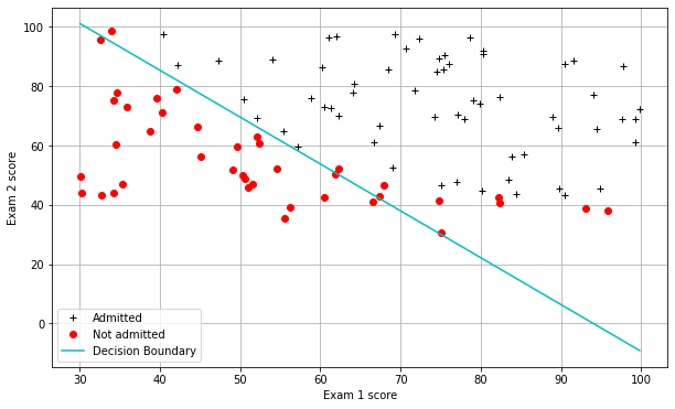
#Plotting the decision boundary: two points, draw a line between
#Decision boundary occurs when h = 0, or when
#theta0 + theta1*x1 + theta2*x2 = 0
#y=mx+b is replaced by x2 = (-1/thetheta2)(theta0 + theta1*x1)

boundary_xs = np.array([np.min(X[:,1]), np.max(X[:,1])])
boundary_ys = (-1./theta[2])*(theta[0] + theta[1]*boundary_xs)
plotData()
plt.plot(boundary_xs,boundary_ys,'c-',label='Decision Boundary')
plt.legend()
<matplotlib.legend.Legend at 0x254f0a1f490>
Lets do it from scratch
import numpy as np
import matplotlib.pyplot as plt
import matplotlib
class LogisticRegression:
"""
A simple class to perform a task of Linear Regression.
Steps
-----
* Find the hypothesis using y = mX + c, where X is as input vector.
* Find the cost value.
* Use gradient descent to update each parameters.
"""
def __init__(self):
"""
This method doesnot take any initial attributes. You will tune the attributes later using methods.
"""
# instantiate train data and label
self.X = None
self.y = None
# to store all costs, initially cost is infinity
self.costs = [np.inf]
# m is for len(X)
self.m = None
# learning rate
self.alpha = None
# our all parameters(from each iterations), m, c in y = mx + c
self.all_parameters = []
def sigmoid(self, x):
return 1 / (1 + np.exp(-x))
def hypothesis(self, x):
"""
A method to perform linear operation(mx + c) and return.
Formula:
--------
\begin{equation}
h{_\theta}{(x)} = {\theta}^{T}x = \theta{_0} + \theta{_1} x_1
\end{equation}
"""
# y = XM, where X is of shape (M, N) and M of (N, 1)
h = self.sigmoid(np.dot(x, self.parameters))
return h
def cost(self, yp, yt):
"""
yp: Predicted y.
yt: True y.
Formula:
-------
\begin{equation}
J{(\theta)} = \frac{1} {2m} \sum_{i=1}^m (h_\theta (x^{(i)}) - y^{(i)})^2
\end{equation}
"""
d = -yt * np.log(yp) - (1 - yt) * np.log(1 - yp)
# finally, sum the square of gradients
delta = np.mean(d)
return delta
def gradient_descent(self):
"""
A method to perform parameter update based on gradient descent algorithm.
Rule:
-----
\begin{equation}
\theta_j = \theta_j - \alpha \frac{1}{m} \sum_{i=1}^m (h_\theta (x^{(i)}) - y^{(i)}) x_j^{(i)}
\end{equation}
"""
temp_theta = self.parameters
# for each theta
for j in range(len(temp_theta)):
# if used square loss
yp = self.hypothesis(self.X)
grad = np.sum((yp - self.y)*yp*(1-yp)*np.array(self.X[:,j]).reshape(self.m, 1))
# if used crossentropy derivative
# grad = np.sum((self.hypothesis(self.X) - self.y)*np.array(self.X[:,j]).reshape(self.m, 1))
temp_theta[j] = self.parameters[j] - (self.alpha / self.m) * grad
self.parameters = temp_theta
self.all_parameters.append(temp_theta.flatten())
def predict(self, X):
"""
A method to return prediction. Perform preprocessing if model was trained preprocessed data.
Preprocessing:
-------------
X = (X - X.mean()) / X.std()
"""
if self.preprocessed != True:
X = np.insert(X,0,1,axis=1)
shape = X.shape
X = np.array([(X[x] - self.means[x+1]) / self.stds[x+1] for x in range(len(X))]).reshape(shape)
return self.hypothesis(X)
def visualize(self, thing="cost"):
"""
Visualise the plots.
Available thing:
----------
i. cost: Cost value vs iteration
ii. param: Parameters vs iteration
iii. all: cost and param vs iteration
"""
legend = ["Loss"]
if thing == "cost" or thing == "all":
plt.title("Loss vs step.")
plt.grid(True)
plt.plot(self.costs)
plt.xlabel("Iterations")
plt.ylabel("Loss")
plt.legend(legend)
#def visualize_parameters(self):
if thing == "param" or thing == "all":
plt.title("Parameter on each step.")
plt.grid(True)
plt.plot(self.all_parameters)
plt.xlabel("Iterations")
plt.ylabel("Parameters")
l = [fr"$\Theta{i}$" for i in range(len(self.parameters))]
if thing == "all":
l.insert(0, legend[0])
legend = l
else:
legend = l
plt.legend(legend)
if thing == "boundary":
self.plotData()
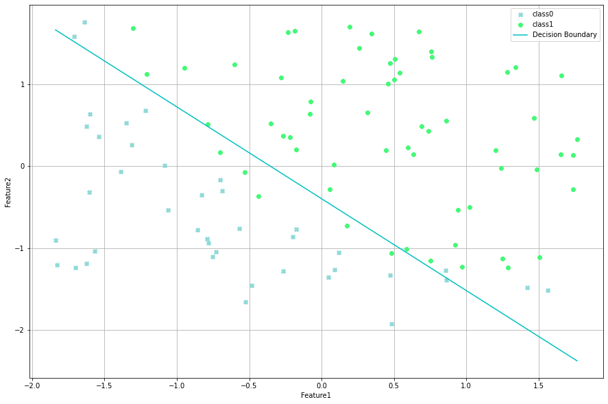
def plotData(self):
"""
Pass non-normalized data.
Assumes X to be of 2 features.
y is ground truth value.
X is train data.
"""
X = self.X
y = self.y
theta = self.parameters
plt.figure(figsize=(15,10))
classes = np.unique(y)
colors = np.random.random(size=(len(classes), 3))
markers = matplotlib.markers.MarkerStyle.markers
lines = matplotlib.lines.lineStyles
_lines = np.array([i for i in list(lines.keys()) if i != "None"])
_markers = np.array([i for i in list(markers.keys()) if i not in ["^", "|", "None", "", " ", None, "_", ","] and
i not in range(12)])
#print(markers)
np.random.shuffle(_lines)
np.random.shuffle(_markers)
#print(_markers)
data = {}
for i, j in zip(X, y):
j = j[0]
if type(data.get(j)) != type(None):
data[j].append(i)
else:
data[j] = [i]
for i, j in enumerate(classes):
plt.plot(np.array(data[j])[:, 1], np.array(data[j])[:, 2], _markers[i], color=colors[i], label=f"class{i}")
boundary_xs = np.array([np.min(X[:,1]), np.max(X[:,1])])
boundary_ys = (-1./theta[2])*(theta[0] + theta[1]*boundary_xs)
plt.plot(boundary_xs,boundary_ys,'c-', label='Decision Boundary')
plt.xlabel('Feature1')
plt.ylabel('Feature2')
plt.legend()
plt.grid(True)
def normalize(self, X):
"""
X: Input training data.
Returns: normalized x.
Normalization:
--------------
X = (X - X.mean()) / X.std()
"""
means, stds = [], []
normalized_x = X.copy()
# since we need to work with only the column we will iterate over shape[1]
for col in range(normalized_x.shape[1]):
means.append(normalized_x[:, col].mean())
stds.append(normalized_x[:, col].std())
if not col: continue
normalized_x[:, col] = (normalized_x[:, col] - means[-1])/stds[-1]
# store the means and stds. We need them on future.
self.means = means
self.stds = stds
return normalized_x
def fit(self, X, y, error_threshold = 0.001, preprocessed = True, alpha=0.01, show_every=100, iterations=1500):
"""
X: input train (m X n), if is not normalized and added axis for bias, use preprocessed=False.
y: train label (n X 1)
error_threshold: How much error is tolerable?
preprocessed: does train data has added axis for bias and normalized?
alpha: learning rate(update step)
show_every: how often to show cost?
iterations: how many steps to run weight update(gradient descent)?
"""
self.preprocessed = preprocessed
# if data already have bias added and normalized, leave it.
if preprocessed!=True:
X = np.insert(X, 0, 1, axis=1)
X = self.normalize(X)
self.X = X
self.y = y
self.alpha = alpha
# how many of training examples are there?
self.m = len(X)
# how many of parameters?
# initialize it to 0, shape must be (num. features + 1, 1)
# X here is normalized i.e it already have axis for bias
self.parameters = np.zeros((X.shape[1], 1))
costs = [np.inf] #Used to plot cost as function of iteration
i = 0
# if our update is not done for iterations and error is pretty high,
while (iterations>i and costs[-1]>error_threshold):
# find the cost value
cost_value = self.cost(self.hypothesis(self.X), self.y)
costs.append(cost_value)
# perform gradient descent and update param
self.gradient_descent()
if i % show_every == 0:
print(f"Step: {i} Cost: {round(cost_value, 4)}.")
i+=1
self.costs = costs
# We have 3 columns and col3 is for prediction of houses
# we need to find mean, std of all the columns
means, stds = [], []
normalized_x = X.copy()
# since we need to work with only the column we will iterate over shape[1]
for col in range(normalized_x.shape[1]):
    means.append(normalized_x[:, col].mean())
    stds.append(normalized_x[:, col].std())
    if not col: continue
    normalized_x[:, col] = (normalized_x[:, col] - means[-1])/stds[-1]
lr = LogisticRegression()

lr.fit(normalized_x[:, :], y, iterations=1500)
# lr.fit(X[:, 1:], y, iterations=150000)
Step: 0 Cost: 0.6931.
Step: 100 Cost: 0.6574.
Step: 200 Cost: 0.6259.
Step: 300 Cost: 0.5984.
Step: 400 Cost: 0.5741.
Step: 500 Cost: 0.5529.
Step: 600 Cost: 0.5341.
Step: 700 Cost: 0.5174.
Step: 800 Cost: 0.5026.
Step: 900 Cost: 0.4893.
Step: 1000 Cost: 0.4773.
Step: 1100 Cost: 0.4665.
Step: 1200 Cost: 0.4566.
Step: 1300 Cost: 0.4476.
Step: 1400 Cost: 0.4394.
lr.visualize(thing="boundary")
Lets use Sklearn now
# import sklearn's logistic regression class
from sklearn.linear_model import LogisticRegression
# create an object of it
model = LogisticRegression()
# fit a model
model.fit(X, y)
C:\ProgramData\Anaconda3\lib\site-packages\sklearn\utils\validation.py:72: DataConversionWarning: A column-vector y was passed when a 1d array was expected. Please change the shape of y to (n_samples, ), for example using ravel().
  return f(**kwargs)


LogisticRegression()
# get model's prediction
mp = model.predict(X)
mp
array([0., 0., 0., 1., 1., 0., 1., 0., 1., 1., 1., 0., 1., 1., 0., 1., 0.,
       0., 1., 1., 0., 1., 0., 0., 1., 1., 1., 1., 0., 0., 1., 1., 0., 0.,
       0., 0., 1., 1., 0., 0., 1., 0., 1., 1., 0., 0., 1., 1., 1., 1., 1.,
       1., 1., 0., 0., 0., 1., 1., 1., 1., 1., 0., 0., 0., 0., 0., 1., 0.,
       1., 1., 0., 1., 1., 1., 1., 1., 1., 1., 0., 1., 1., 1., 1., 0., 1.,
       1., 0., 1., 1., 0., 1., 1., 0., 1., 1., 1., 1., 1., 0., 1.])
# get our model's predictions
# we will round it to nearest int to get exact class
op = np.round(lr.predict(normalized_x)).reshape(1, -1)
op[0]
array([0., 0., 0., 1., 1., 0., 1., 0., 1., 1., 1., 0., 1., 1., 0., 1., 0.,
       0., 1., 1., 0., 1., 0., 0., 1., 1., 1., 1., 0., 0., 1., 1., 0., 0.,
       0., 0., 1., 1., 0., 0., 1., 0., 1., 0., 0., 0., 1., 1., 1., 1., 1.,
       1., 1., 0., 0., 0., 1., 1., 1., 1., 1., 0., 0., 0., 0., 0., 1., 0.,
       1., 1., 0., 1., 1., 1., 1., 1., 1., 1., 0., 1., 1., 1., 1., 0., 1.,
       1., 0., 1., 1., 0., 1., 1., 0., 1., 1., 1., 1., 1., 0., 1.])
# get mse between these two predictions
mse = np.mean((mp-op[0])**2)
mse
0.01
# get mse between our model and true y
mse1 = np.mean((y-op[0])**2)
mse1
0.48
# get mse between sklearn model and true y
mse2 = np.mean((y-mp)**2)
mse2
0.478
# the mse are not that far in fact the difference on error is  little
abs(mse1-mse2)
0.0020000000000000018
Finally
The class we proposed is not that bad and when comparing the mse of our scratch model and the mse of sklearn’s model, difference on mse is little. But on the production level, using frameworks is a best way.
Why not read more?
- Linear Regression from Scratch
- Writing Popular ML Optimizers from Scratch
- Feed Forward Neural Network from Scratch
- Convolutional Neural Networks from Scratch
- Writing a Simple Image Processing Class from Scratch
- Deploying a RASA Chatbot on Android using Unity3d
- Gesture Based Visually Writing System Using OpenCV and Python
- Naive Bayes for text classifications: Scratch to Framework
- Simple OCR for Devanagari Handwritten Text


Comments