
Auto-encoders from Scratch in Python
Auto-encoders from scratch build on the same neural network fundamentals I covered earlier. If you haven’t already, see these prerequisite posts:
I also wrote about data encoding techniques such as Run Length Encoding from Scratch.
I started drafting this post in May 2020 but paused after completing the neural-network tutorials. In November 2022 I received a helpful reader email that motivated me to finish it.

What is an auto-encoder?
An auto-encoder is a neural network trained to reconstruct its input. It has two logical parts:
- Encoder — compresses the input into a lower-dimensional representation (the bottleneck or latent vector).
- Decoder — reconstructs the original input from that compressed representation.
The network learns an implicit “key” in its weights (the parameters) that maps inputs to compressed representations and back.
Unlike typical supervised learning, auto-encoders are often intentionally driven to overfit training data in order to learn detailed reconstructions. However, depending on the use case (denoising, compression, anomaly detection) you may want to regularize or constrain the latent space.
Applications and intuition
Auto-encoders are useful for several tasks:
- Dimensionality reduction and compression (store a small latent vector instead of the original data).
- Denoising (train the model to remove noise from inputs).
- Anomaly detection (anomalous inputs typically reconstruct poorly, producing higher loss).
- Colorization or modality translation (e.g., grayscale → RGB using encoder/decoder pairs).
A conceptual example: train an auto-encoder on a collection of high-resolution images so the encoder produces a compact code you can store and the decoder can later reconstruct the image. The model weights and architecture become critical — you must persist them to reconstruct images later.
Code (from my Quark library)
The implementation below uses my custom package Quark. You can find the project on GitHub:
Imports
from quark.layers import *
from quark.Stackker import Sequential
import pandas as pd
import matplotlib.pyplot as plt
Load MNIST
Note: corrected spelling from “minst” to “MNIST”.
from keras.datasets import mnist
(x_train, y_train), (x_test, y_test) = mnist.load_data()
Preprocess
Flatten and normalize pixel values to [0,1]. For this auto-encoder the target is the input itself.
x = x_train.reshape(-1, 28 * 28) / 255.0
xt = x_test.reshape(-1, 28 * 28) / 255.0
Build and train a simple auto-encoder
This example uses three fully connected layers: an encoder layer, a small hidden layer, and a decoder that reconstructs the input.
m = Sequential()
m.add(FFL(784, 10, activation='sigmoid'))
m.add(FFL(10, 10, activation='relu'))
m.add(FFL(10, 784, activation='sigmoid'))
m.compile_model(lr=0.001, opt="adam", loss="mse")
m.summary()
m.train(x, x, epochs=10, batch_size=32, val_x=xt, val_y=xt)
A typical model summary and training output looks like this:
Input  Output Shape Activation  Bias  Parameters
...
Total Parameters: 16584

Validation data found.
Total 60000 samples.
Training samples: 60000 Validation samples: 10000.

Epoch: 0:
Time: 97.376sec
Train Loss: 0.0674 Train Accuracy: 0.1443%
Val Loss: 0.0675 Val Accuracy: 0.1441%

...
Note: accuracy in an auto-encoder is not a meaningful metric for pixel-wise reconstruction — focus on reconstruction loss (MSE) instead. You may also see a RuntimeWarning from the sigmoid implementation if very large inputs are passed to the exponential; proper weight initialization or using ReLU in hidden layers typically prevents extreme values.
Training on my machine took ~23 minutes for 10 epochs. The loss decreased steadily even though the “accuracy” numbers remain low; that is expected for this task.
Visualize reconstructions
fig, axes = plt.subplots(nrows=2, ncols=10, sharex=True, sharey=True, figsize=(20,4))
in_imgs = xt[:10]
reconstructed = m.predict(in_imgs)
for images, row in zip([in_imgs, reconstructed], axes):
    for img, ax in zip(images, row):
        ax.imshow(img.reshape((28, 28)), cmap='Greys_r')
        ax.get_xaxis().set_visible(False)
        ax.get_yaxis().set_visible(False)
fig.tight_layout(pad=0.1)
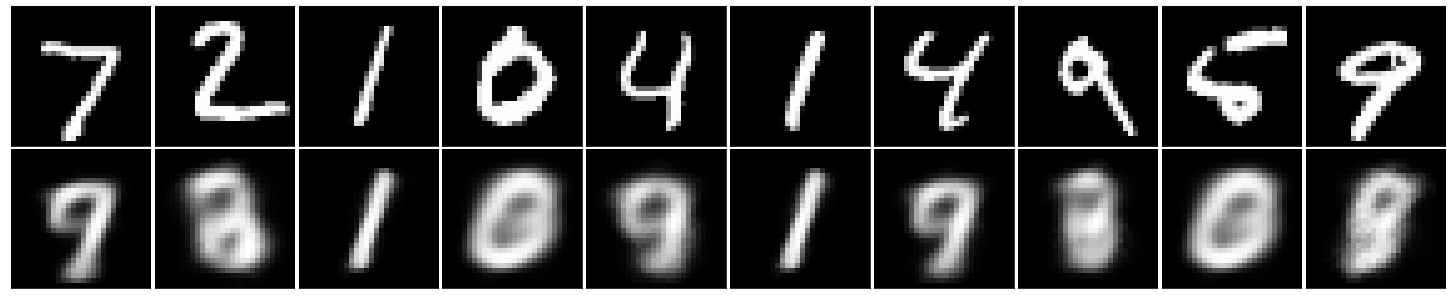
The reconstructed images resemble the inputs, but they are not perfect. Training longer, changing the architecture, or using convolutional layers would likely improve visual quality.
Notes, improvements and next steps
- Use convolutional auto-encoders (Conv-AEs) for image tasks — they preserve spatial structure and generally produce better reconstructions.
- Add a bottleneck with fewer neurons to force a more compact latent representation.
- Try different loss functions (e.g., binary cross-entropy for normalized pixels) or perceptual losses for visually better reconstructions.
- Implement denoising auto-encoders by adding noise to inputs and training the model to predict the clean images.
- Save and version model weights and architecture when relying on reconstructed outputs as compressed storage.
Conclusion
We implemented and trained a simple auto-encoder from scratch using a custom neural-network package and MNIST. This post demonstrates the basic idea and provides directions for improving the model (convolutions, bottlenecking, denoising, and different losses). I hope you find it useful.
If you’d like, I can:
- Replace the fully connected model with a convolutional auto-encoder example.
- Add code to save/load model weights and demonstrate compression ratio calculations.
- Show a denoising auto-encoder variant with example noisy inputs.


Comments