Beyond EDA: Taking Exploratory Data Analysis into Machine Learning Modelling with Python

Exploratory Data Analysis, or EDA, helps us understand a dataset. It tells us what the data looks like, which columns are important, how features are distributed, which variables are correlated, and whether there are patterns worth exploring.

But EDA is not the final step.

After we understand the data, we often want to use that knowledge for modelling. This can mean:

• clustering similar data points
• predicting a numeric value
• classifying data into categories
• testing whether EDA insights can become a useful machine learning model

This post is a continuation of the earlier blog:

• A General Way of Doing EDA

In the previous post, we explored an IoT telemetry dataset. In this post, we will take that EDA knowledge and move toward machine learning modelling.

What This Tutorial Covers

We will cover:

• how EDA connects to modelling
• reading and preparing IoT telemetry data
• using EDA findings as modelling ideas
• K-Means clustering
• elbow method for choosing clusters
• K-Medoids clustering
• linear regression
• multiple linear regression
• voting regression
• neural network regression
• logistic regression classification
• decision tree classification
• neural network classification
• practical lessons from modelling

The goal is not only to train models, but also to understand why we choose each method.

From EDA to Modelling

EDA gives us clues.

For example:

• if two features are strongly correlated, regression may be useful
• if data points form visible groups, clustering may be useful
• if we have a known label, classification may be useful
• if simple models are not enough, more complex models may be tested

The main question is:

Can the patterns found during EDA be turned into useful predictions or decisions?

A few examples:

EDA Insight	Possible Action
Sweets sell more in December	Stock more sweets before December
Sales increase after marketing	Predict next campaign sales
Customers show different spending patterns	Cluster customers into groups
Sensor values differ by device location	Classify device location from readings
LPG, smoke, and CO are strongly related	Predict CO using LPG and smoke

EDA helps us ask better modelling questions.

What We Knew from EDA

From the earlier EDA, we had a few important findings:

• ANOVA suggested that sensor readings differ significantly by device.
• Some fields had strong correlations for specific devices.
• LPG, smoke, and CO were highly related.
• The three devices appeared to be placed in different environmental conditions.

The devices were interpreted like this:

Device	Environmental condition
00:0f:00:70:91:0a	cooler and more humid
1c:bf:ce:15:ec:4d	variable temperature and humidity
b8:27:eb:bf:9d:51	stable, warmer, and dryer

Now we will use this information for modelling.

Reading the Data

First, import the required libraries.

from datetime import datetime

import matplotlib.pyplot as plt
import numpy as np
import pandas as pd
import seaborn as sns

from sklearn.cluster import KMeans
from sklearn.ensemble import GradientBoostingRegressor, RandomForestRegressor, VotingRegressor
from sklearn.linear_model import LinearRegression, LogisticRegression
from sklearn.metrics import accuracy_score, confusion_matrix, f1_score, mean_squared_error, r2_score
from sklearn.model_selection import GridSearchCV, train_test_split
from sklearn.preprocessing import StandardScaler
from sklearn.tree import DecisionTreeClassifier

Optional imports:

try:
    from sklearn_extra.cluster import KMedoids
    HAS_KMEDOIDS = True
except ImportError:
    HAS_KMEDOIDS = False

Now read the dataset.

df = pd.read_csv("iot_telemetry_data.csv")

Convert timestamp into datetime.

df["date"] = df["ts"].apply(datetime.fromtimestamp)

Add readable device names.

device_names = {
    "00:0f:00:70:91:0a": "cooler, more humid",
    "1c:bf:ce:15:ec:4d": "variable temp/humidity",
    "b8:27:eb:bf:9d:51": "stable, warmer, dry",
}

df["device_name"] = df["device"].map(device_names)

Preview the data.

df.head()

The dataset contains columns such as:

• ts
• device
• co
• humidity
• light
• lpg
• motion
• smoke
• temp
• date
• device_name

Feature Columns

For modelling, we will use sensor columns.

feature_cols = [
    "co",
    "humidity",
    "light",
    "lpg",
    "motion",
    "smoke",
    "temp",
]

Some columns are boolean, such as light and motion. scikit-learn can handle boolean values after conversion, but it is often cleaner to convert them to integers.

df["light"] = df["light"].astype(int)
df["motion"] = df["motion"].astype(int)

Clustering

Clustering is an unsupervised learning method. It tries to group similar data points without using labels.

In this dataset, we already know that the data comes from three devices. But clustering can help us test whether the sensor readings naturally form groups.

We will start with:

• K-Means
• K-Medoids

K-Means Clustering

K-Means tries to divide data into k clusters.

The basic idea is:

1. choose k cluster centers
2. assign each data point to the nearest center
3. update each center based on assigned points
4. repeat until cluster assignments become stable

K-Means works well when clusters are roughly circular and distance-based grouping makes sense.

K-Means with Two Features

Let us start with two features:

cols = ["co", "temp"]
X = df[cols]

Train K-Means with three clusters.

kmeans = KMeans(
    n_clusters=3,
    random_state=42,
    n_init="auto"
)

df["cluster"] = kmeans.fit_predict(X)

Now plot the result.

def scatterplot(data, x, y, hue, figsize=(15, 10), title=None, centers=None):
    plt.figure(figsize=figsize)

    sns.scatterplot(
        data=data,
        x=x,
        y=y,
        hue=hue,
        s=10
    )

    if centers is not None:
        plt.scatter(
            centers[:, 0],
            centers[:, 1],
            c="black",
            s=200,
            alpha=0.6,
            label="Centers"
        )

    if title is None:
        title = f"{x} vs {y} by {hue}"

    plt.title(title, fontsize=20)
    plt.xlabel(x, fontsize=14)
    plt.ylabel(y, fontsize=14)
    plt.legend()
    plt.show()

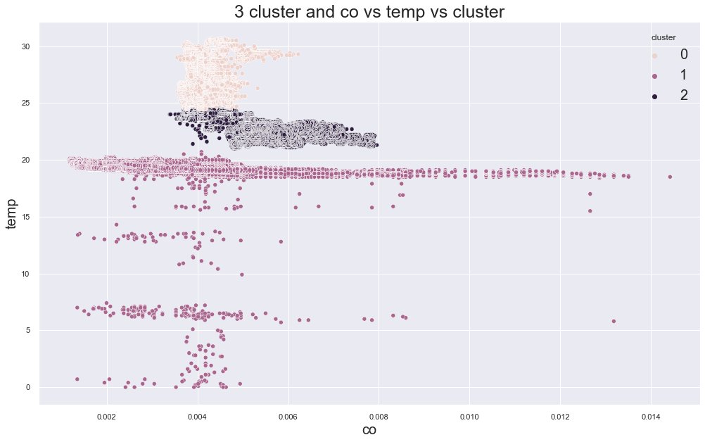
scatterplot(
    data=df,
    x="co",
    y="temp",
    hue="cluster",
    centers=kmeans.cluster_centers_
)

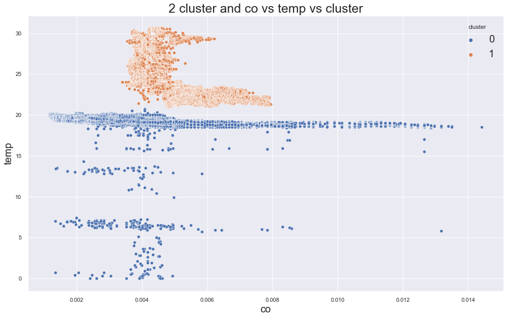
Output:

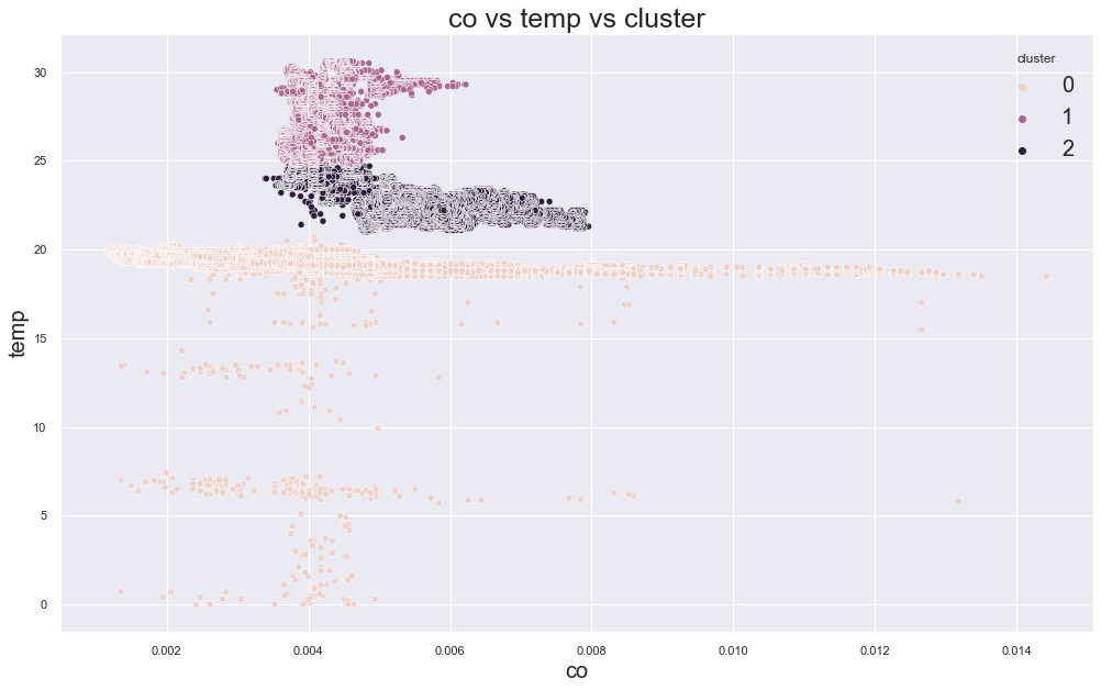
There seems to be some clustering, but we need to check whether those clusters are meaningful.

Check Cluster Meaning

df.groupby("cluster")["device_name"].value_counts()

In the original experiment, one device appeared across several clusters. That means the clusters were not perfectly matching the device locations.

This is an important lesson:

A cluster can look visible in a plot, but still not be meaningful for the real-world question.

Elbow Method for K-Means

To choose the number of clusters, we can use the elbow method.

cols = ["co", "temp"]
X = df[cols]

errors = []
cluster_range = range(2, 10)

for k in cluster_range:
    model = KMeans(
        n_clusters=k,
        random_state=42,
        n_init="auto"
    )

    model.fit(X)
    errors.append(model.inertia_)

Plot the error.

plt.figure(figsize=(15, 10))
plt.plot(cluster_range, errors, "bx-")
plt.xlabel("Values of K")
plt.ylabel("Inertia")
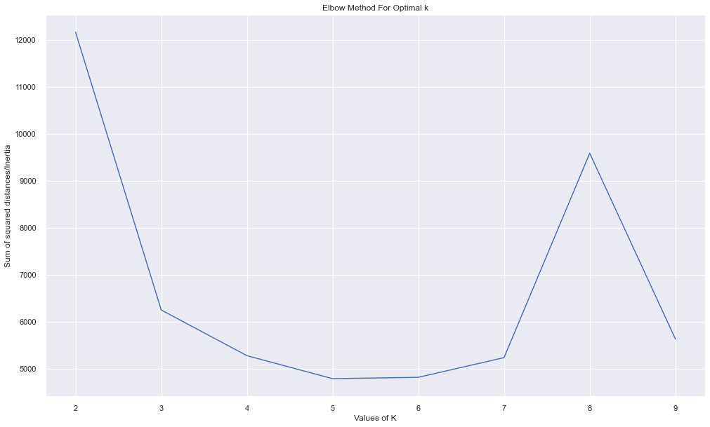
plt.title("Elbow Method for Optimal K")
plt.show()

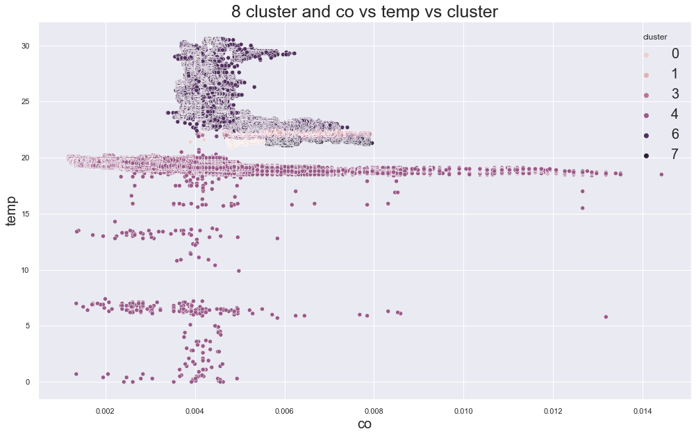
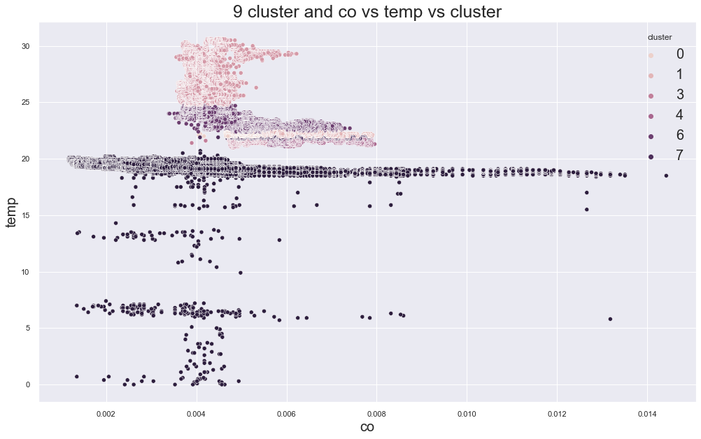
Output:

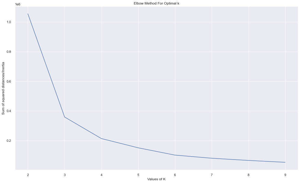
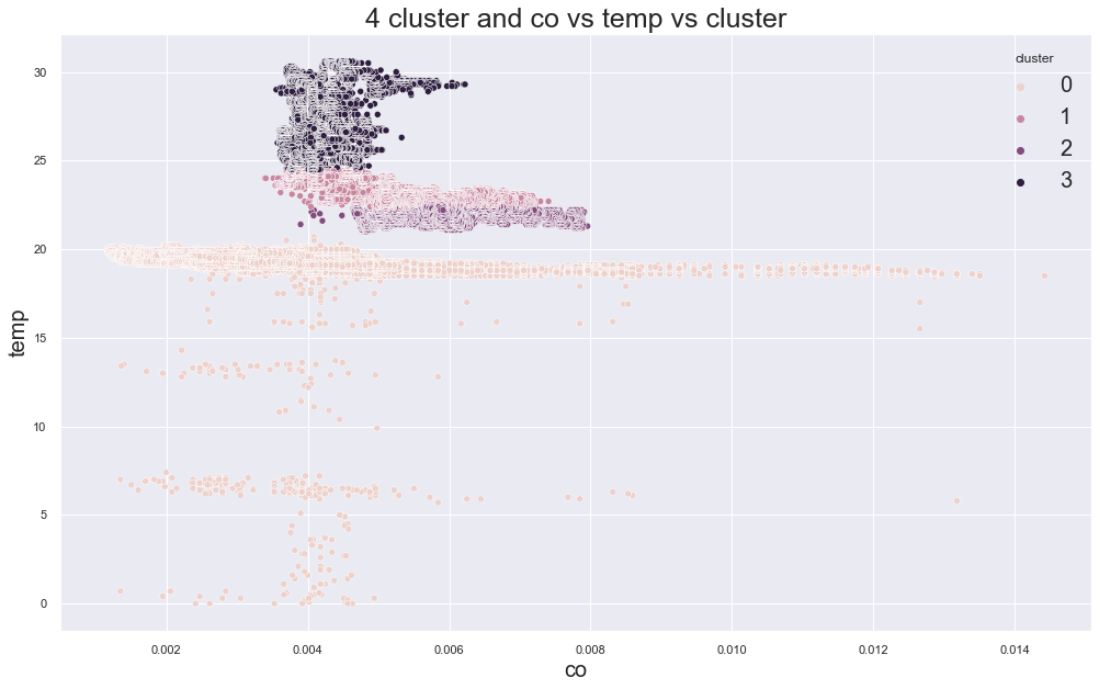
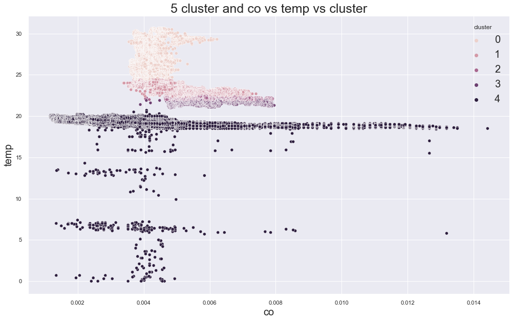
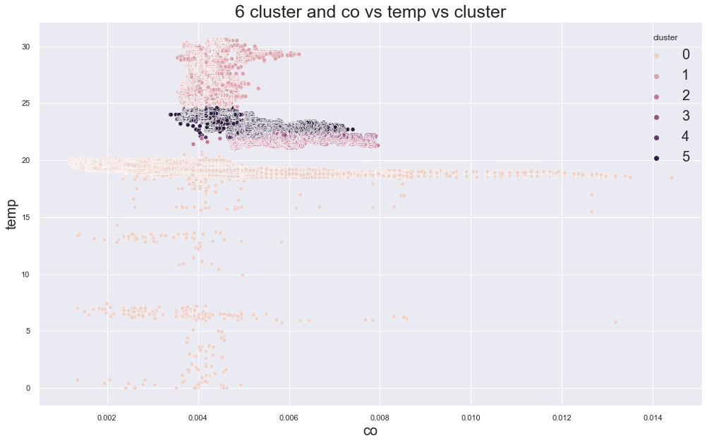
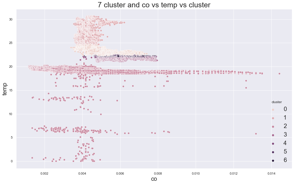
In the original result, k=3 or k=4 looked reasonable because the error decreased strongly before that point.

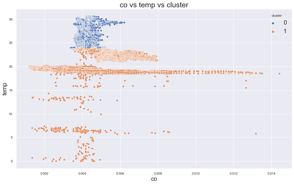
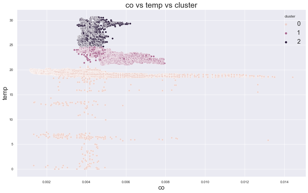
Example outputs from different K values:

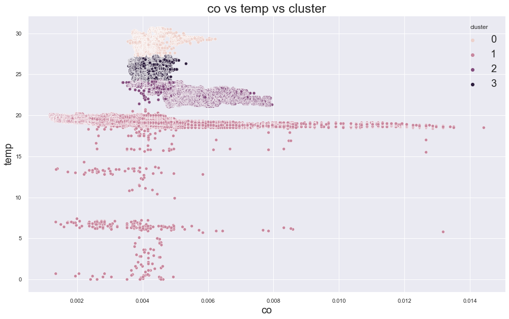
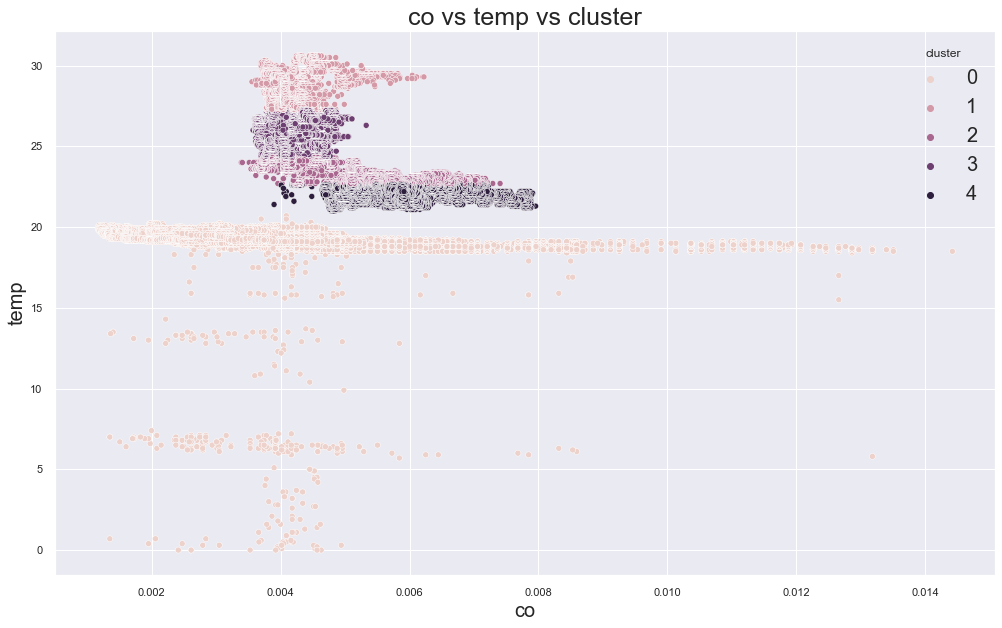
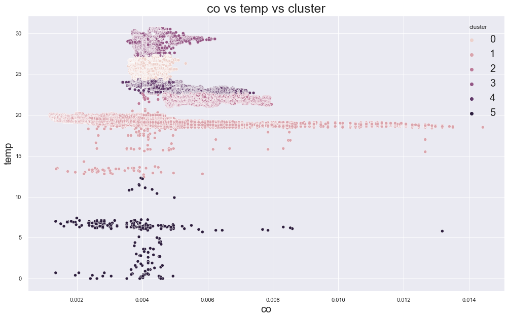
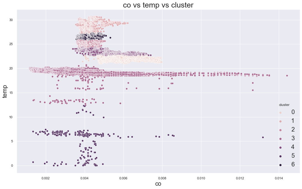
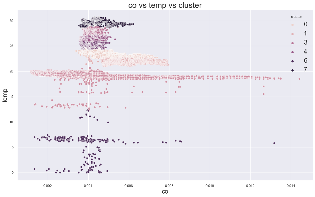
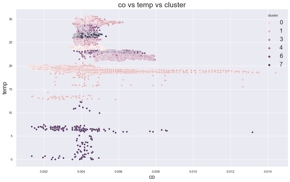
K-Medoids Clustering

K-Medoids is similar to K-Means, but instead of using mean points as centers, it uses actual data points as cluster centers.

Those center points are called medoids.

K-Medoids can be more robust to outliers than K-Means, but it can be slower and more memory-heavy.

Install it with:

pip install scikit-learn-extra

Then use:

from sklearn_extra.cluster import KMedoids

K-Medoids on Sample Data

Because the dataset is large, it is better to fit K-Medoids on a sample.

cols = ["co", "temp"]
X = df[cols]

sample_X = X.sample(
    n=10000,
    random_state=42
)

kmedoids = KMedoids(
    n_clusters=3,
    random_state=42,
    metric="manhattan"
)

kmedoids.fit(sample_X)

df["cluster"] = kmedoids.predict(X)

Now plot the result.

scatterplot(
    data=df,
    x="co",
    y="temp",
    hue="cluster",
    title="K-Medoids Clustering"
)

Example outputs:

K-Medoids elbow plot:

In the original experiment, K-Medoids also suggested around three clusters, but the device groups were still not perfectly separated.

Clustering Lesson

Clustering did not fully separate the devices based only on co and temp.

This can happen because:

• two features may not capture the full pattern
• devices may overlap in sensor readings
• one device may have more variable conditions
• time-related patterns may be important
• clustering does not know the real labels

So, clustering is useful for exploration, but it should not be trusted blindly.

Regression

Regression is used when we want to predict a numeric value.

In this dataset, EDA showed strong relationships between:

• LPG
• smoke
• CO

So, we can try to predict co from lpg and smoke.

Simple Linear Regression

A simple linear regression has the form:

\[y = mx + c\]

Where:

• y is the dependent variable
• x is the independent variable
• m is the slope
• c is the intercept

Here, we will predict co from lpg.

X = df[["lpg"]]
y = df["co"]

model = LinearRegression()
model.fit(X, y)

pred = model.predict(X)

print("Intercept:", model.intercept_)
print("Slope:", model.coef_)

Plot the result.

plt.figure(figsize=(15, 10))
plt.scatter(X, y, color="red", s=5, alpha=0.4)
plt.plot(X, pred, color="blue")
plt.xlabel("LPG")
plt.ylabel("CO")
plt.title("LPG vs CO: Original and Predicted")
plt.legend(["Predicted", "Original"])
plt.show()

Output:

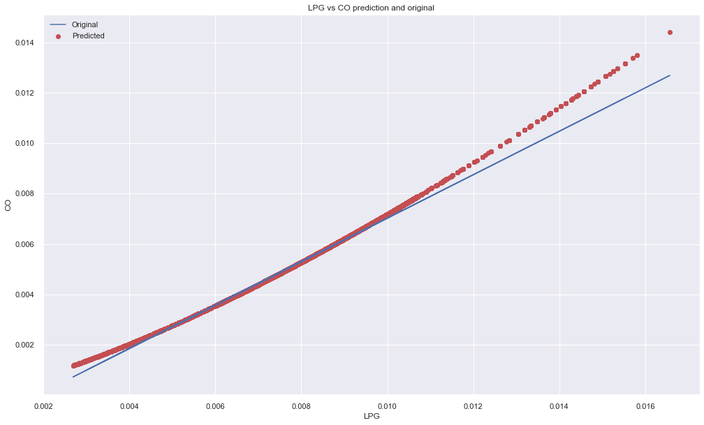
The line fits some parts well because LPG and CO are strongly related.

Regression Metrics

Two useful regression metrics are:

• Mean Squared Error
• R2 Score

mse = mean_squared_error(y, pred)
r2 = r2_score(y, pred)

print("MSE:", mse)
print("R2:", r2)

Mean Squared Error measures average squared prediction error.

R2 score tells how much of the variance in the target can be explained by the model. A perfect R2 score is 1.0. It can also be negative if the model is worse than a simple baseline.

Multiple Linear Regression

Now use both lpg and smoke to predict co.

X = df[["lpg", "smoke"]]
y = df["co"]

model = LinearRegression()
model.fit(X, y)

pred = model.predict(X)

print("Intercept:", model.intercept_)
print("Coefficients:", model.coef_)

print("MSE:", mean_squared_error(y, pred))
print("R2:", r2_score(y, pred))

The equation is:

\[y = \beta_0 + \beta_1x_1 + \beta_2x_2\]

In this case:

• y is CO
• x1 is LPG
• x2 is smoke

The original experiment showed a very high R2 score because these gas-related variables are strongly related.

Voting Regression

Voting regression trains multiple regression models and averages their predictions.

Here we use:

• Gradient Boosting Regressor
• Random Forest Regressor
• Linear Regression

X = df[["lpg", "smoke"]]
y = df["co"]

reg1 = GradientBoostingRegressor(random_state=1)
reg2 = RandomForestRegressor(random_state=1, n_estimators=50)
reg3 = LinearRegression()

voting_regressor = VotingRegressor([
    ("gb", reg1),
    ("rf", reg2),
    ("lr", reg3),
])

models = {
    "Gradient Boosting": reg1,
    "Random Forest": reg2,
    "Linear Regression": reg3,
    "Voting Regressor": voting_regressor,
}

Train and compare:

for name, model in models.items():
    model.fit(X, y)
    pred = model.predict(X)

    print(name)
    print("MSE:", mean_squared_error(y, pred))
    print("R2:", r2_score(y, pred))
    print()

In the original experiment, all models performed well, but Random Forest had a very small MSE.

Neural Network Regression

Neural networks can also be used for regression.

A neural network learns by:

1. passing input forward
2. computing output
3. comparing output with target
4. calculating loss
5. backpropagating error
6. updating weights

The simplest neural network is related to the idea of a perceptron.

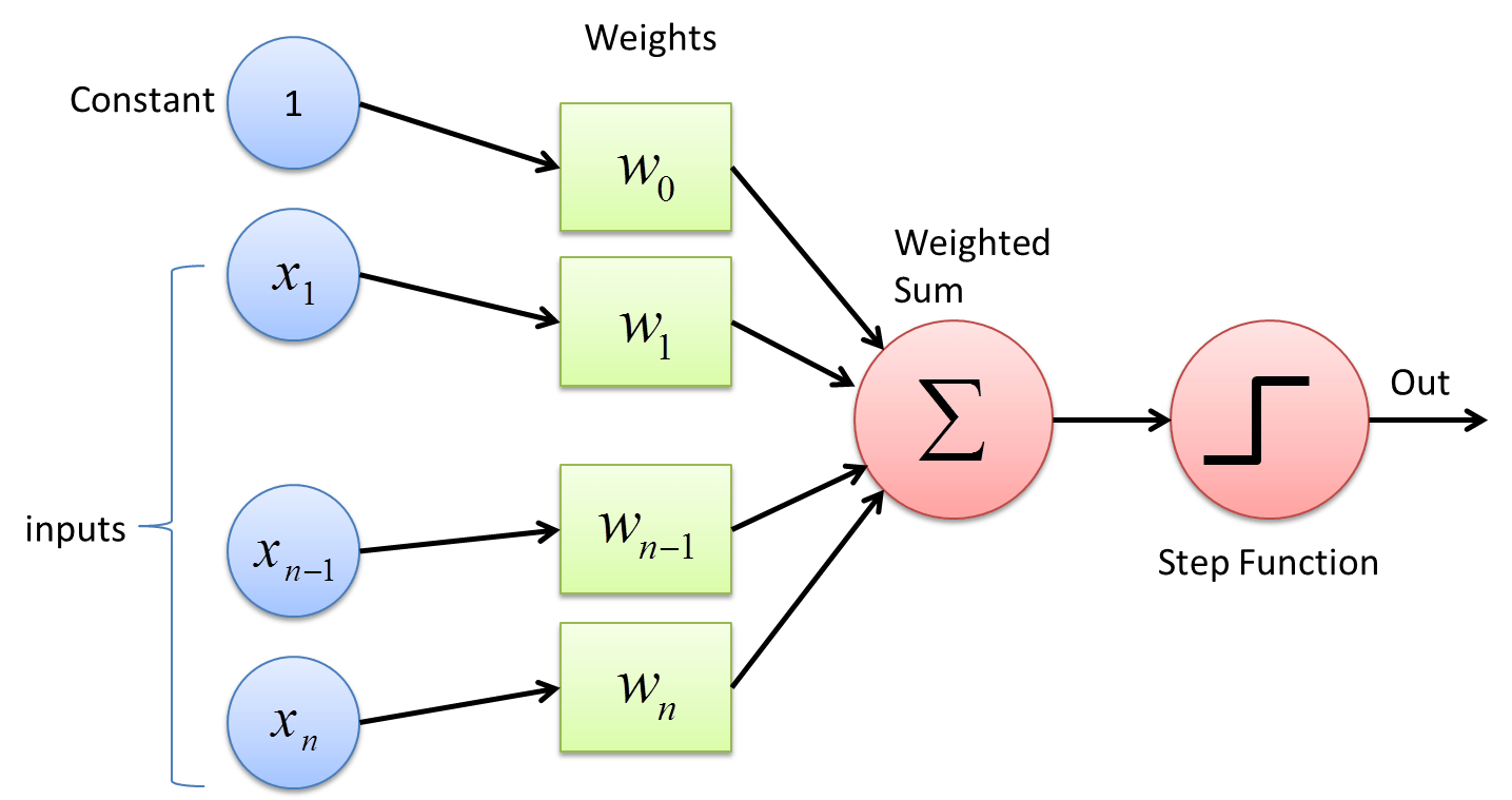
Referenced from deepai.org.

Simple Keras Regression Model

import tensorflow as tf
from tensorflow.keras import Sequential
from tensorflow.keras.layers import Dense

Prepare data:

X = df[["lpg", "smoke"]].to_numpy().astype("float32")
y = df["co"].to_numpy().astype("float32")

Build a simple model:

model = Sequential([
    Dense(8, activation="relu", input_shape=(X.shape[1],)),
    Dense(4, activation="relu"),
    Dense(1),
])

model.compile(
    optimizer="adam",
    loss="mse"
)

history = model.fit(
    X,
    y,
    epochs=5,
    validation_split=0.2,
    batch_size=256
)

Plot training loss.

plt.plot(history.history["loss"])
plt.plot(history.history["val_loss"])
plt.title("Model Loss")
plt.ylabel("Loss")
plt.xlabel("Epoch")
plt.legend(["train", "val"], loc="upper left")
plt.show()

Original neural network regression outputs:

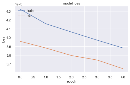
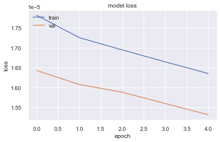
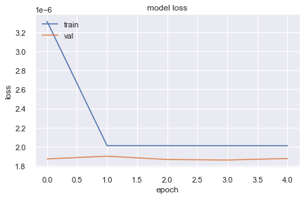
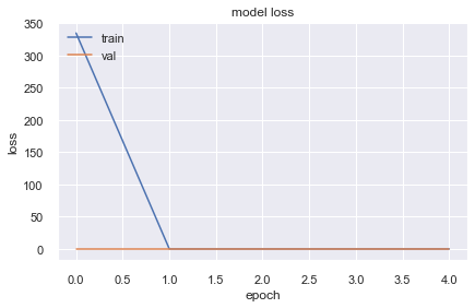
Neural Network Regression Lesson

The original experiment showed that the neural network loss did not always improve better than simple models.

This is an important lesson:

Neural networks are powerful, but they are not automatically better for every dataset.

Neural networks may perform poorly if:

• the data is not scaled
• the architecture is not suitable
• the optimizer is not suitable
• the data is small or too simple
• the target has a simple linear relationship
• the training setup is not tuned

For this CO prediction task, simpler models were already strong.

Classification

Classification is used when we want to predict categories.

In this dataset, we can predict which device produced a reading.

There are three device classes:

device_to_label = {
    "00:0f:00:70:91:0a": 0,
    "1c:bf:ce:15:ec:4d": 1,
    "b8:27:eb:bf:9d:51": 2,
}

df["y"] = df["device"].map(device_to_label)

Features:

xcols = ["co", "humidity", "light", "lpg", "motion", "smoke", "temp"]

X = df[xcols]
y = df["y"]

Split the data:

X_train, X_test, y_train, y_test = train_test_split(
    X,
    y,
    test_size=0.2,
    random_state=42,
    stratify=y
)

Scale features:

scaler = StandardScaler()

X_train_scaled = scaler.fit_transform(X_train)
X_test_scaled = scaler.transform(X_test)

Logistic Regression

Logistic Regression is a classification algorithm. Despite the name, it is commonly used for classification, not regression.

It works well for binary classification, but it can also handle multi-class classification.

clf = LogisticRegression(
    max_iter=1000,
    multi_class="auto"
)

clf.fit(X_train_scaled, y_train)

pred = clf.predict(X_test_scaled)

print("Accuracy:", accuracy_score(y_test, pred))
print("F1:", f1_score(y_test, pred, average="macro"))

In the original experiment, Logistic Regression achieved very high accuracy.

Grid Search for Logistic Regression

Grid Search trains the same model with different hyperparameters and selects the best one using cross-validation.

parameters = {
    "C": [0.001, 0.01, 0.1, 1, 10, 100],
    "penalty": ["l2"],
}

grid_search = GridSearchCV(
    estimator=LogisticRegression(max_iter=1000),
    param_grid=parameters,
    scoring="accuracy",
    cv=5,
    n_jobs=-1
)

grid_search.fit(X_train_scaled, y_train)

print("Best Accuracy:", grid_search.best_score_)
print("Best Parameters:", grid_search.best_params_)

Predict using the best model.

best_model = grid_search.best_estimator_
pred = best_model.predict(X_test_scaled)

print("Test Accuracy:", accuracy_score(y_test, pred))
print("Test F1:", f1_score(y_test, pred, average="macro"))

Confusion Matrix

A confusion matrix shows how many samples were classified correctly or incorrectly.

cm = confusion_matrix(y_test, pred)

sns.heatmap(
    cm,
    annot=True,
    fmt="d",
    cmap="Blues"
)

plt.xlabel("Predicted")
plt.ylabel("Actual")
plt.title("Confusion Matrix")
plt.show()

Original output:

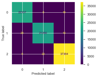
Only a few samples were misclassified in the original experiment.

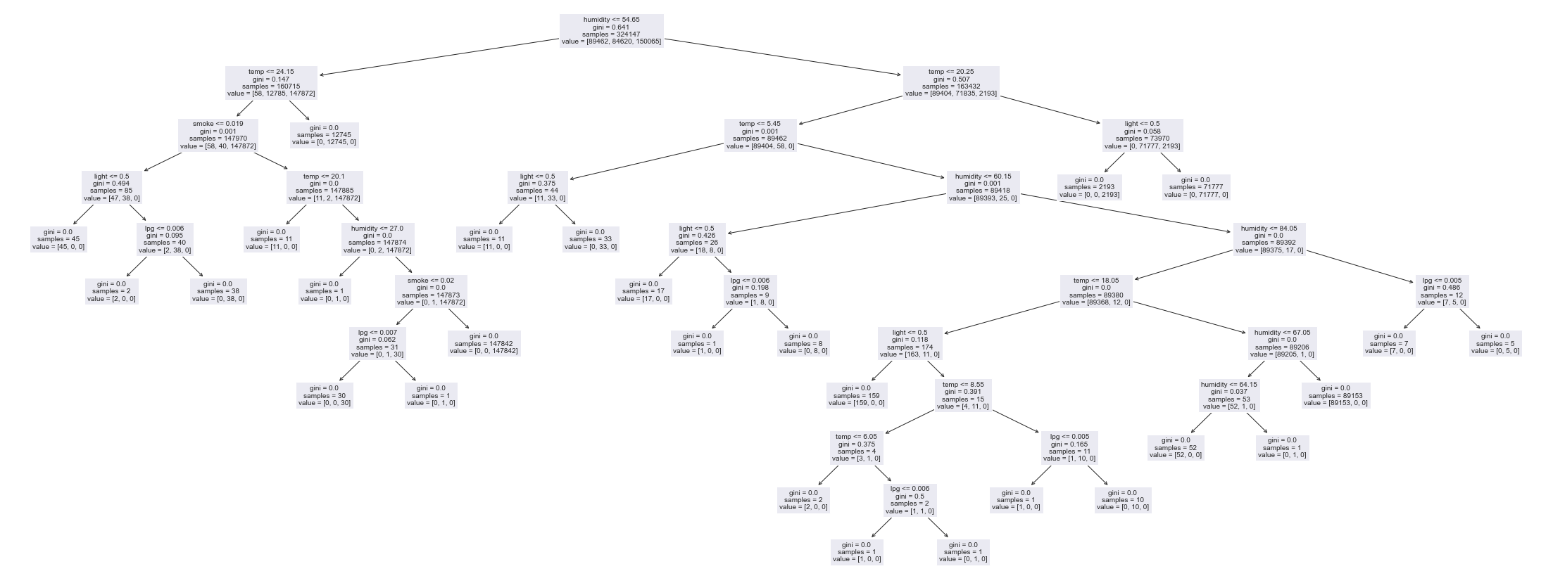
Decision Tree Classifier

Decision Trees work like a series of if-else decisions.

tree_clf = DecisionTreeClassifier(
    random_state=42
)

tree_clf.fit(X_train, y_train)

tree_pred = tree_clf.predict(X_test)

print("Accuracy:", accuracy_score(y_test, tree_pred))
print("F1:", f1_score(y_test, tree_pred, average="macro"))

The original Decision Tree also performed extremely well.

Visualize the tree.

from sklearn import tree

plt.figure(figsize=(35, 15))
tree.plot_tree(
    tree_clf,
    feature_names=xcols,
    class_names=["device_0", "device_1", "device_2"],
    filled=True,
    fontsize=10
)
plt.show()

Original tree output:

Neural Network Classification

For multi-class classification, a neural network can use:

• softmax activation in the output layer
• sparse_categorical_crossentropy loss for integer labels

Prepare data:

X = df[xcols].to_numpy().astype("float32")
y = df["y"].to_numpy().astype("int64")

X_train, X_test, y_train, y_test = train_test_split(
    X,
    y,
    test_size=0.2,
    random_state=42,
    stratify=y
)

scaler = StandardScaler()

X_train = scaler.fit_transform(X_train)
X_test = scaler.transform(X_test)

Build model:

model = Sequential([
    Dense(16, activation="relu", input_shape=(X_train.shape[1],)),
    Dense(8, activation="relu"),
    Dense(3, activation="softmax"),
])

model.compile(
    optimizer="adam",
    loss="sparse_categorical_crossentropy",
    metrics=["accuracy"]
)

history = model.fit(
    X_train,
    y_train,
    epochs=10,
    validation_split=0.2,
    batch_size=256
)

Evaluate:

test_loss, test_acc = model.evaluate(X_test, y_test)

print("Test loss:", test_loss)
print("Test accuracy:", test_acc)

Plot performance.

plt.figure(figsize=(15, 10))
plt.plot(history.history["loss"])
plt.plot(history.history["accuracy"])
plt.plot(history.history["val_loss"])
plt.plot(history.history["val_accuracy"])
plt.title("Model Performance")
plt.ylabel("Value")
plt.xlabel("Epoch")
plt.legend(
    ["train_loss", "train_acc", "val_loss", "val_acc"],
    loc="upper left"
)
plt.show()

Original neural network classification output:

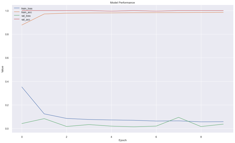
Classification Lessons

The classification models performed very well because the device environments were highly distinct.

However, very high accuracy should always be checked carefully.

Possible reasons for very high accuracy:

• classes are naturally easy to separate
• train and test data are very similar
• data leakage exists
• one or more features directly identify the class
• the split is random but the data is time-dependent

For time-series or sensor data, random train-test split may be too optimistic. A time-based split can be more realistic.

Better Validation for Sensor Data

For sensor data, validation should be chosen carefully.

Useful validation methods:

Method	Use Case
Random split	quick baseline
Stratified split	class-balanced classification
Time-based split	future prediction
Group-based split	avoid same device/session leakage
Cross-validation	robust model comparison

For this dataset, if the goal is to classify device type from sensor values, random split may be fine as a first experiment. If the goal is future deployment, time-based validation is better.

Full Modelling Workflow

A good workflow after EDA is:

1. define the modelling question
2. choose target variable
3. choose features
4. split data properly
5. preprocess data
6. train simple baseline model
7. evaluate with proper metrics
8. compare with stronger models
9. check errors
10. validate assumptions
11. decide whether the model is useful

EDA should not be separate from modelling. It should guide modelling.

Common Mistakes

Mistake 1: Using Clustering Without Meaning

Clusters should be interpreted with domain knowledge. A colorful plot does not always mean useful groups.

Mistake 2: Trusting High Accuracy Too Quickly

Very high accuracy can be real, but it can also happen because of leakage or easy labels.

Mistake 3: Not Scaling Features

Many models perform better when features are scaled.

Examples:

• Logistic Regression
• K-Means
• Neural Networks
• KNN
• SVM

Mistake 4: Using Neural Networks Too Early

Start with simple models first. If simple models work well, a neural network may not be necessary.

Mistake 5: Ignoring Time

Sensor data is often time-dependent. Random splits may not always represent real deployment.

Practical Conclusions

From this experiment:

• EDA gave useful clues about device differences.
• K-Means and K-Medoids showed some grouping, but not perfect separation with only two features.
• LPG and smoke were strong predictors of CO.
• Linear models worked well for gas-related variables.
• Random Forest regression performed very well in the original experiment.
• Logistic Regression and Decision Trees classified devices with high accuracy.
• Neural networks worked, but required more care and were not automatically better.
• Model selection depends on data, target, features, and validation strategy.

Final Thoughts

In this blog, we moved beyond EDA into modelling. We used insights from exploratory data analysis to test clustering, regression, classification, and neural networks on IoT telemetry data.

The main lesson is simple:

EDA should guide modelling, but modelling should also challenge EDA assumptions.

A pattern seen in EDA is not automatically a useful model. We still need proper validation, metrics, and domain understanding.

Start with simple models, understand the errors, and only then move to more complex methods.