Python for Stock Market Analysis: Growth Rates

Introduction

Interactive plot version of blog is available at here.

This is the part 3 of our Python for Stock Market Analysis series and here, we will explore some of popular growth rates that can be used to see how well is our value is changing over the period of time. Lets take some of scenarios:

• If we want to know by what rate is our current month’s closing price is changed compared to the previous, we could simply divide change of values by the values at base month.
• If we want to know the compounding change rate of our closing price compared to the base period.
• We want to predict how much will the growth rate be on the next month or to achieve the constant growth rate, what should be the value.

The scenarios can be many more but lets focus on some.

Again we will be using the data reading part’s code from the previous blogs.

import pandas as pd
import numpy as np
import plotly.express as px
import cufflinks
import plotly.io as pio 
import yfinance as yf
import warnings 
warnings.filterwarnings("ignore")
cufflinks.go_offline()
cufflinks.set_config_file(world_readable=True, theme='pearl')
pio.renderers.default = "notebook"

pd.options.display.max_columns = None

symbols = ["AAPL"]

df = yf.download(tickers=symbols)
# convert column names into lowercase
df.columns = [c.lower() for c in df.columns]
df.rename(columns={"adj close":"adj_close"},inplace=True)

df.head()

	open	high	low	close	adj_close	volume
Date
1980-12-12	0.128348	0.128906	0.128348	0.128348	0.100323	469033600
1980-12-15	0.122210	0.122210	0.121652	0.121652	0.095089	175884800
1980-12-16	0.113281	0.113281	0.112723	0.112723	0.088110	105728000
1980-12-17	0.115513	0.116071	0.115513	0.115513	0.090291	86441600
1980-12-18	0.118862	0.119420	0.118862	0.118862	0.092908	73449600

Rate of Return

Lets suppose that we bought a stock 2 months ago and we want to find out how much profit we currently have then we might subtract the price at the time we bought from the current price. And it can be simply called return. The rate of return is simple measurement that tells us how much has been the price increase from the base period. It is calculated as:

\[ror = \frac{V_{current}-V_{initial}}{V_{initial}} * 100\]

RoR is the simplest growth rate and it does not take external factors like inflation into consideration.

mdf["ror"] = 100*(mdf.Close-mdf.Close.tolist()[0])/mdf.Close.tolist()[0]


mdf.iplot(kind="line", x="Date",y="ror", title="Rate of Return")

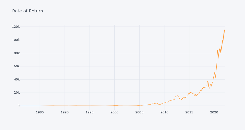
Looking over above plot, the rate of return is more than 100K and it is not much useful for new buyers. New buyers might need to look into latest data’s ROR or ROR from last few years only. Or even from some period.

Windowed ROR

So, lets take a window of 12 and calculate rate of return in that period. Because this way, we will be considering only latest points while calculating the ROR.

window=12
mdf[f"wror_{window}"] = 0
idxs = mdf.index.tolist()
for idx in [idxs[i-window:i] for i in range(window, len(idxs)+1)]:
    tmp = mdf.iloc[mdf.index.isin(idx)].Close.tolist()
    ror = (tmp[-1]-tmp[0])/tmp[0]
    i = idx[-1]
    mdf.loc[i, f"wror_{window}"] = ror*100
mdf.iplot(kind="line", x="Date", y=[f"wror_{window}"])

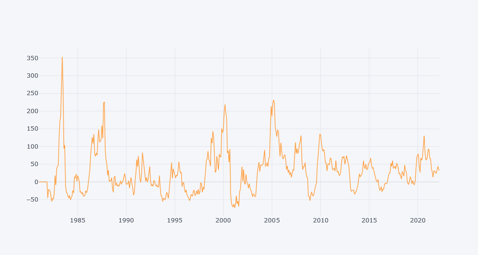
Now it is making little bit more sense.

Month Over Month (MOM) Growth Rate

This is the simple measurement of the growth rate where we simply calculate the rate of change from the previous month.

\[rate = \frac{v_t - v_{t-1}}{v_{t-1}} * 100\]

Where,

• v(t) is value at month t.
• v(t-1) is value at month t-1.

Lets calculate this in our python. But first, lets make a dataframe to store the closing price of the month only.

mdf = df.resample("1M").close.last().rename("Close").reset_index()
mdf["momgr"] = mdf.Close.pct_change()*100
mdf

	Date	Close	momgr
0	1980-12-31	0.152344	NaN
1	1981-01-31	0.126116	-17.216307
2	1981-02-28	0.118304	-6.194292
3	1981-03-31	0.109375	-7.547504
4	1981-04-30	0.126674	15.816225
...	...	...	...
491	2021-11-30	165.300003	10.347129
492	2021-12-31	177.570007	7.422870
493	2022-01-31	174.779999	-1.571216
494	2022-02-28	165.119995	-5.526950
495	2022-03-31	173.041000	4.797121

import plotly.graph_objects as go
from plotly.subplots import make_subplots

fig=make_subplots(specs=[[{"secondary_y": True}]])


lastn = 100
ldf = mdf[-lastn:]

fig.add_trace(go.Line(x=ldf.Date, y=ldf.momgr, line=dict(
                color='rgb(104, 14, 24)',

            ), 
              name="MOM Growth Rate Closing Price"),secondary_y=True)
fig.add_trace(go.Line(x=ldf.Date, y=ldf.Close, line=dict(
                color='rgb(10, 104, 204)',), 
              name="MOM Closing Price"),secondary_y=False)


fig.update_layout(
    title= "AAPL Stock Data",
    yaxis_title="MOM Growth Rate Closing Price",
    xaxis_title="Date")               
fig.update_yaxes(title_text="MOM Closing Price", secondary_y=False)
fig.update_yaxes(title_text="MOM Growth Rate Closing Price", secondary_y=True)

fig.show()

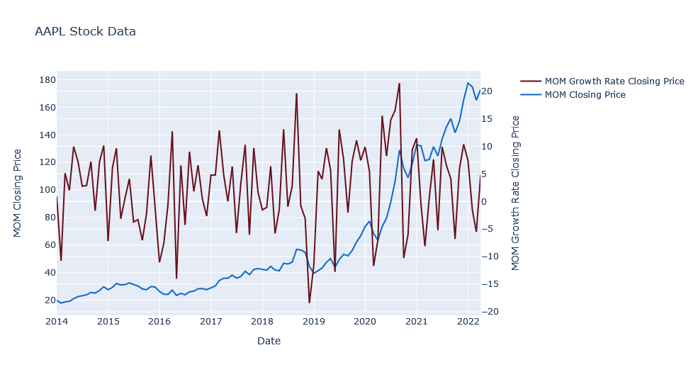
Looking over the data of last 100 months, we have used MOM closing price on the primary y axis while MOM growth rate is on secondary y axis. The Growth rate does not seem to be increasing but is fluctuating.

Compounding Monthly Growth Rate (CMGR)

Compounding monthly growth rate is the rate of closing price that would be required for an stock’s closing price to grow from its base closing to its ending closing price. And it can be calculated as:

\[CMGR = \left[\left(\frac{V_{t}}{V_0} \right)^{\frac{1}{n}} - 1\right]*100\]

Where,

• V0 is first observation or observation at base period and Vt is observation at time t.
• n is number of months from base month to t.

Since this growth rate is compounding, we can calculate this in entire history of the closing prices or calculate on the some moving window like in 5 months.

Simple CGR

Lets take a value at the first month as the base value.

mdf["n"] = np.arange(0,len(mdf))
mdf["cmgr"] = ((mdf.Close  / mdf.Close[0]) ** (1/mdf["n"]) - 1) * 100
mdf.iplot(kind="line", x="Date", y="cmgr", title=f"CMGR % of AAPL")

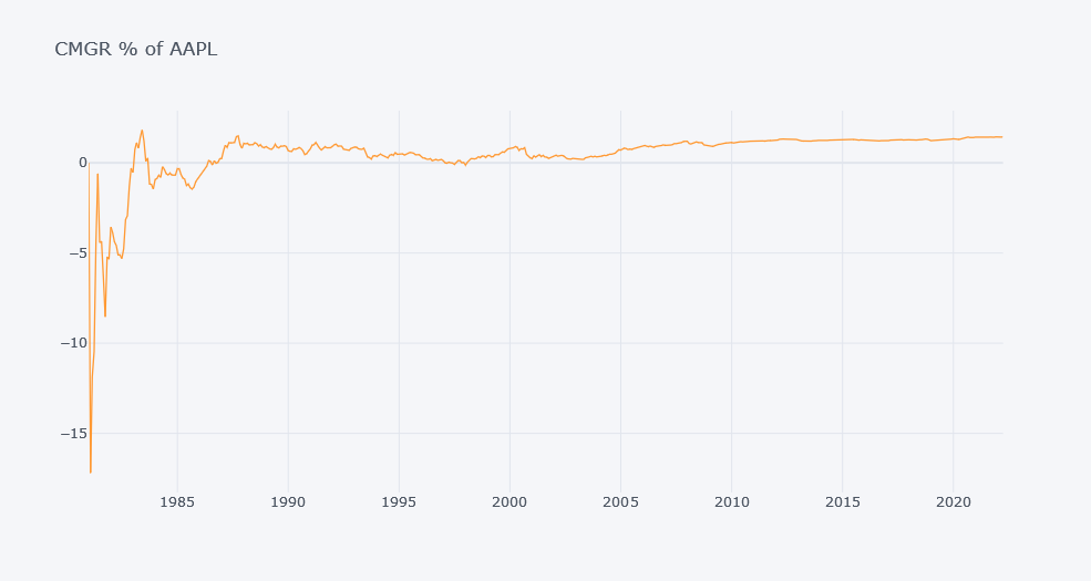
Looking over the above plot, there seems to have huge loss in closing price before 1990 but looking over the latest dates, there seems to be having positive but low growth rates.

It might not be always an good idea to look over the CMGR by taking initial value of closing price as a base value but we could select a window over which we will calculate a CMGR so that we could compare the Growth in that window only. This can be thought as, we bought a stock today and our base day will be today. And while calculating CMGR, we will take closing value of today.

Windowed CMGR

In this part, we will calculate the growth rate in some time period only but not from the beginning. So lets find indices for each window. In below code block, we took all the index of mdf and then looped over the each chunk of indices of size equal to the value of window.

window=12
mdf[f"wcmgr_{window}"] = 0
idxs = mdf.index.tolist()
for idx in [idxs[i-window:i] for i in range(window, len(idxs)+1)]:
    tmp = mdf.iloc[mdf.index.isin(idx)].Close.tolist()
    wcmgr = (tmp[-1]/tmp[0])**(1/window)-1
    i = idx[-1]
    mdf.loc[i, f"wcmgr_{window}"] = wcmgr*100
mdf.iplot(kind="line", x="Date", y=[f"wcmgr_{window}", "cmgr"])

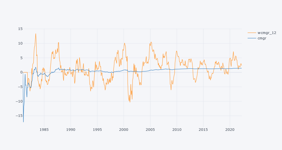
Looking over the above plot, one can make some sense like:

• The overall simple CMGR is increasing slowly.
• The Windowed GR is alo increasing but it has lots of ups and downs because of having multiple base periods.

Year over Year (YoY) Growth Rate

adf = df.resample("1Y").close.last().rename("Close").reset_index()
adf["yoygr"] = adf.Close.pct_change()*100
adf

import plotly.graph_objects as go
from plotly.subplots import make_subplots

fig=make_subplots(specs=[[{"secondary_y": True}]])


lastn = 100
ldf = adf[-lastn:]

fig.add_trace(go.Line(x=ldf.Date, y=ldf.yoygr, line=dict(
                color='rgb(104, 14, 24)',

            ), 
              name="YoY Growth Rate Closing Price"),secondary_y=True)
fig.add_trace(go.Line(x=ldf.Date, y=ldf.Close, line=dict(
                color='rgb(10, 104, 204)',), 
              name="YoY Closing Price"),secondary_y=False)


fig.update_layout(
    title= "AAPL Stock Data",
    yaxis_title="YoY Growth Rate Closing Price",
    xaxis_title="Date")               
fig.update_yaxes(title_text="YoY Closing Price", secondary_y=False)
fig.update_yaxes(title_text="YoY Growth Rate Closing Price", secondary_y=True)

fig.show()

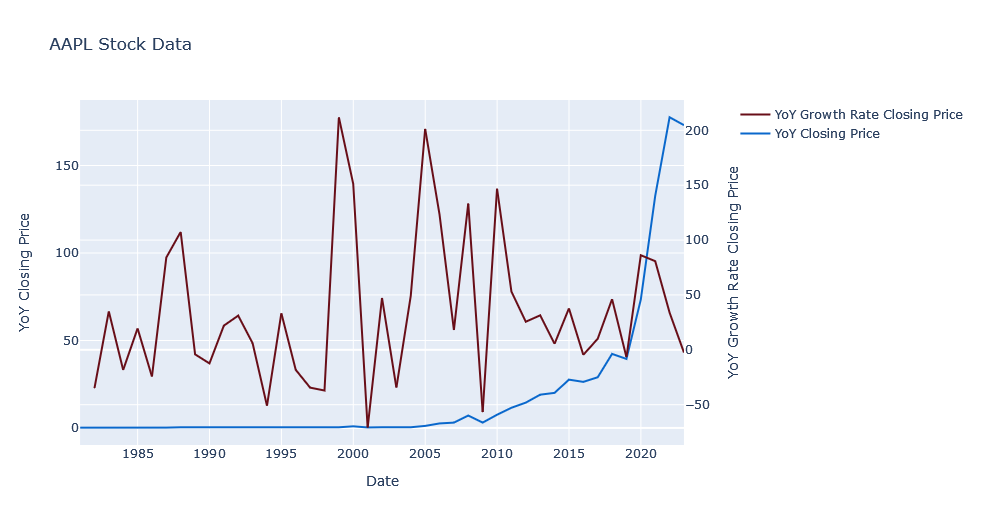
Looking over the plot above, YoYGR seems to be increasing but what about Compounding Growth?

Compounding Annual Growth Rate (CAGR)

It is simply a modified version of CMGR. In CMGR, we calculate rates based on the month while in CAGR, we do same for the year. So, lets create a dataframe for annual closing prices.

Simple CAGR

adf["n"] = np.arange(0,len(adf))
adf["cagr"] = ((adf.Close  / adf.Close[0]) ** (1/adf["n"]) - 1) * 100
adf.iplot(kind="line", x="Date", y="cagr", title=f"CAGR % of AAPL")

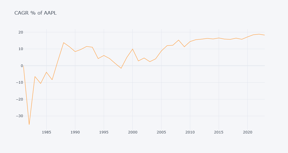
CAGR Seems to be increasing but CMGR did not give us an insight as strong as this one. Since CMGR looks over only month’s data, growth rate could be small in that little time.

Windowed CAGR

Lets look over the 5 window year’s CAGR.

window=5
adf[f"wcagr_{window}"] = 0
idxs = adf.index.tolist()
for idx in [idxs[i-window:i] for i in range(window, len(idxs)+1)]:
    tmp = adf.iloc[adf.index.isin(idx)].Close.tolist()
    wcagr = (tmp[-1]/tmp[0])**(1/window)-1
    i = idx[-1]
    adf.loc[i, f"wcagr_{window}"] = wcagr*100
adf.iplot(kind="line", x="Date", y=[f"wcagr_{window}", "cagr"])

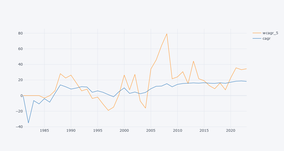
Using a window gave us pretty bad result but it might be because our window is small.

window=10
adf[f"wcagr_{window}"] = 0
idxs = adf.index.tolist()
for idx in [idxs[i-window:i] for i in range(window, len(idxs)+1)]:
    tmp = adf.iloc[adf.index.isin(idx)].Close.tolist()
    wcagr = (tmp[-1]/tmp[0])**(1/window)-1
    i = idx[-1]
    adf.loc[i, f"wcagr_{window}"] = wcagr*100
adf.iplot(kind="line", x="Date", y=[f"wcagr_{window}", "cagr"])

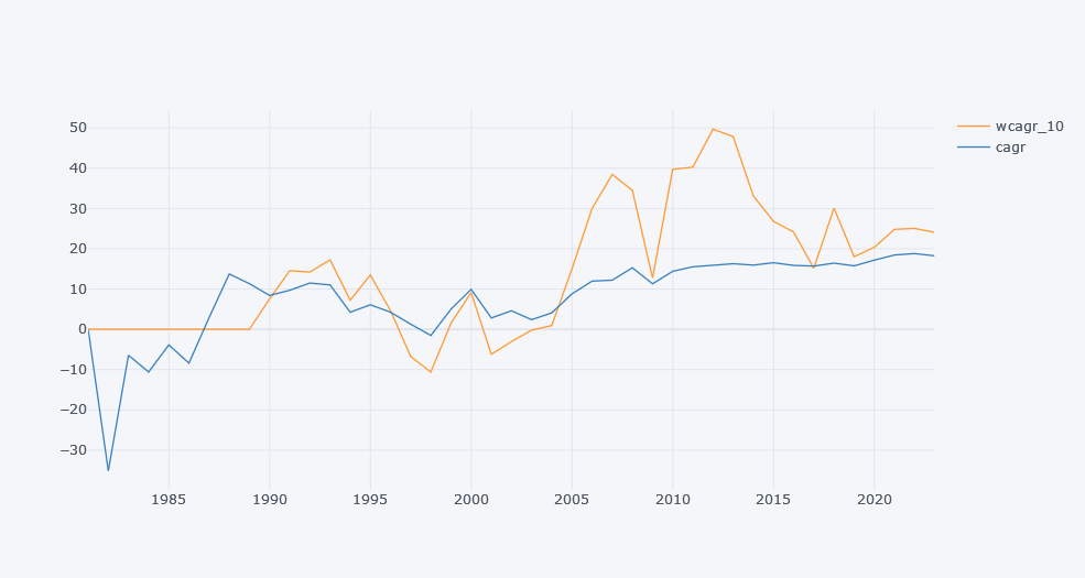
Now it is nearly identical to the CAGR. If we kept adding window size, it will eventually become a CAGR.

Thank you everyone for reading this blog. Please stay tuned for the next one.

References

• CAGR-Investopedia