
Central Tendency vs Dispersion
Hello everyone, welcome back! In this blog we will again focus into the some of widely used central tendency techniques and then measure of spread in the Statistical Analysis of the EDA part. If you are looking for a brief walk-through of a Statistical Data Analysis in Data Science please refer to this blog of mine.
Central Tendency
Central tendency in statistics is the property of a data which tries to explain the central portion of the data. There are different types of the central tendency and each have their advantage and disadvantages. Lets explore them below.
We will calculate these values in the the titanic dataset.
Mean
Mean is the most common measure of a central tendency where we divide the sum of all data points by the number of the data points. This is often called as an average and is denoted by Greek symbol $\mu$.
import numpy as np
import pandas as pd
import seaborn as sns

df = pd.read_csv("https://raw.githubusercontent.com/datasciencedojo/datasets/master/titanic.csv")
df.head()
| PassengerId | Survived | Pclass | Name | Sex | Age | SibSp | Parch | Ticket | Fare | Cabin | Embarked | |
|---|---|---|---|---|---|---|---|---|---|---|---|---|
| 0 | 1 | 0 | 3 | Braund, Mr. Owen Harris | male | 22.0 | 1 | 0 | A/5 21171 | 7.2500 | NaN | S |
| 1 | 2 | 1 | 1 | Cumings, Mrs. John Bradley (Florence Briggs Thayer) | female | 38.0 | 1 | 0 | PC 17599 | 71.2833 | C85 | C |
| 2 | 3 | 1 | 3 | Heikkinen, Miss. Laina | female | 26.0 | 0 | 0 | STON/O2. 3101282 | 7.9250 | NaN | S |
| 3 | 4 | 1 | 1 | Futrelle, Mrs. Jacques Heath (Lily May Peel) | female | 35.0 | 1 | 0 | 113803 | 53.1000 | C123 | S |
| 4 | 5 | 0 | 3 | Allen, Mr. William Henry | male | 35.0 | 0 | 0 | 373450 | 8.0500 | NaN | S |
</div>
df.Age.mean()
29.69911764705882
The mean age of the passenger seems to be 29.6.
Median
Median in statistics is the point of data which is exactly in the center of the data when it is sorted. Median should cut the data points into two halves. Median is often called as second quartile and is calculated as (where N is number of data point):
-
When N is odd, \(\text{median} = \left(\frac{N+1}{2} \right)^{th} \text{item}\)
-
When N is even,
df.Age.median()
28.0
But the median age of the customer seems to be 28.
Mode
Mode is the value which is most repeated in the data.
df.Age.mode()
0    24.0
dtype: float64
Age 24 seems to have repeated most. But is it true?
df.Age.value_counts().sort_values(ascending=False)
24.00    30
22.00    27
18.00    26
28.00    25
19.00    25
         ..
0.67      1
20.50     1
66.00     1
24.50     1
12.00     1
Name: Age, Length: 88, dtype: int64
Yes, it is. It seems that there are 30 passengers with age 24. Which is the most repeated.
Quartiles
Besides mean, median and mode, quartiles are also sometimes taken along with median. Quartiles gives the values which lies in the 25, 50 and the 75 percentile of the data. But data has to be sorted first.
df.Age.describe()
count    714.000000
mean      29.699118
std       14.526497
min        0.420000
25%       20.125000
50%       28.000000
75%       38.000000
max       80.000000
Name: Age, dtype: float64
Looking over the quartile values above, we can see that the minimum value is 0.42, 25% is 20, median or 50% is 28, mean is 29 and 75% is 38 and max is 80. It seems that our data is slightly spread, as max value is far from the 3rd quartile.
Box Plot
sns.boxplot(data=df, x="Age")
<AxesSubplot:xlabel='Age'>
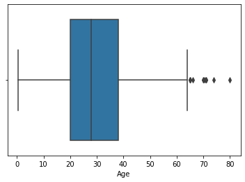
Box plot gives the values just like pandas describe. It seems that most of the data are within our 3rd quartile.
Mid Range
This is not considered exactly as the central tendency but still it is useful to see how far is our average from the mid range. Mid Range gives the average of the highest and lowest value on the series. Which is simply an arithmetic mean.
(df.Age.min() + df.Age.max())/2
40.21
It seems that our mid range age is 40.21.
When to use what?
- If the data is normally distributed, that is the mean is exactly in the center.
- We should use median rather than mean when there is huge outliers in the data. Because the mean gets skewed towards direction of outliers but not the median.
Dispersion
Dispersion is a measure of the spread in the data. It is often used along with the central tendency and sometimes it depends on the central tendency too.
Inter Quartile Range (IQR)
It is the difference between Q3 and Q1.
df.Age.quantile(0.75)-df.Age.quantile(0.25)
17.875
It seems that our two quartiles are not much far. Which represents that, majority of the data is around center and this is good in the sense of outliers.
Range
It is the simplest measure of the dispersion, where we subtract smallest value from the largest value. This gives the idea of how huge is our data difference is.
df.Age.max()-df.Age.min()
79.58
It seems that the maximum difference between value is 79.58 but our IQR was only 17.875. There are certainly outliers in the data.
Standard Deviation
It is the measure of the distance between each points of data with the mean data. This is most widely used measurement of the dispersion because this often gives the error in the data points. \(s = \sqrt{\dfrac{\sum_{i=1}^{n}(x_i - \overline{x})^{2}}{n}}\)
df.Age.std()
14.526497332334044
Z-Score
This answers the question How many standard deviation away is the data from the mean? It is calculated as:
Where,
- x is the estimation of the mean or raw score
- 𝜇 is the population mean
- 𝜎 is the population standard deviation
Z Score is often used to compare the mean of two different samples and examine which is better than another. Lets take an example of comparing z score. A scored 172 in x and 50 on 37 on y. While mean and std for x and y are (151, 10) and (25.1, 6.4) resp. Z score for both is, 2.1, 1.86. We can conclude that, A scored relatively better in x than y. Lets do this in our Age by taking 500 random samples from our data and comparing it with our population z score.
pop = df.Age
sample1 = df.Age.sample(500)
sample2 = df.Age.sample(500)
sample1_z = (pop.mean()-sample1.mean())/pop.std()
sample2_z = (pop.mean()-sample2.mean())/pop.std()
sample1_z, sample2_z
(0.030374493169490115, 0.020496044621050025)
Looking over above two sample’s z scores, we can say that the mean age of sample two is slightly nearer towards the population mean.
When to use what?
- If we are about to compare means from two different population then we should be using z score.
- If we are about to look how huge data points are, then simple range should be used.
- For looking into how far are the mid points of two halves are, IQR should be used.
- For measuring how far is each data point is from the mean value, Standard Deviation is used.
Shifting and Scaling of Mean and Standard Deviation
- Mean shifts by same amount as the data shift(add) amount.
- Mean increases by amount as the data was increased by amount.
- Median has property as same as of mean for shift and scale.
- Standard deviation does not shift but scales by amount.
- IQR has same property as of standard deviation.
Lets verify above properties. First calculate the describe of age and then another describe by multiplying age by 2.
df.Age.describe()
count    714.000000
mean      29.699118
std       14.526497
min        0.420000
25%       20.125000
50%       28.000000
75%       38.000000
max       80.000000
Name: Age, dtype: float64
(2*df.Age).describe()
count    714.000000
mean      59.398235
std       29.052995
min        0.840000
25%       40.250000
50%       56.000000
75%       76.000000
max      160.000000
Name: Age, dtype: float64
It seems that, mean and standard deviation has been increased by 2 times. But lets see what happens when we shift the data by 5 points.
(2+df.Age).describe()
count    714.000000
mean      31.699118
std       14.526497
min        2.420000
25%       22.125000
50%       30.000000
75%       40.000000
max       82.000000
Name: Age, dtype: float64
It seems that our means has been shifted but the standard deviation has not changed. Thus we can say that, the shift and the scaling property of dispersion and central tendency is different.


Comments