OpenCV Image Processing in Python: Beginner Guide with Examples

OpenCV is one of the most popular libraries for image processing and computer vision. It provides many tools for reading images, changing color spaces, filtering, thresholding, edge detection, contour detection, video processing, face detection, and even deep learning-based object detection.

This post is an introduction to OpenCV image processing in Python. I originally wrote this notebook in 2019 when I was just learning computer vision. I have now cleaned it up, improved the explanations, and made it easier to follow as a beginner tutorial.

Note: Some example images used in the original notebook were collected from the internet when I was learning. Credit belongs to the original image authors.

What This Tutorial Covers

In this OpenCV Python tutorial, we will cover:

• OpenCV installation
• image representation
• image reading and display
• BGR vs RGB color channels
• grayscale conversion
• image transforms
• image masking
• image filtering
• high-pass and low-pass filters
• image thresholding
• Canny edge detection
• Hough transform for line detection
• Haar cascade face detection
• contours
• color tracking with HSV
• a short introduction to YOLO object detection with OpenCV DNN

What Is OpenCV?

OpenCV stands for Open Source Computer Vision Library. It was originally written in C and C++, but it can now be used from Python, Java, Android, C#, and other platforms.

OpenCV can be used for many computer vision tasks, such as:

• reading and writing images
• reading videos and webcams
• image resizing and rotation
• image filtering and blurring
• image thresholding
• edge detection
• contour detection
• object tracking
• face detection
• feature detection
• camera calibration
• deep learning inference with DNN models

For Python users, OpenCV is usually imported as cv2.

Install OpenCV in Python

You can install OpenCV with pip:

pip install opencv-python

If you also need extra modules, you can install:

pip install opencv-contrib-python

For most beginner image processing tasks, opencv-python is enough.

Import Required Packages

import cv2
import numpy as np
import matplotlib.pyplot as plt

print(cv2.__version__)

We use:

• cv2 for OpenCV operations
• numpy because images are stored as arrays
• matplotlib to display images in notebooks

Image Representation

A digital image is stored as a grid of pixels. Each pixel contains intensity values.

For an 8-bit grayscale image:

• 0 means black
• 255 means white
• values between 0 and 255 represent different gray levels

For a color image, each pixel usually contains three values:

• Red
• Green
• Blue

A color image with shape (100, 100, 3) has:

100 rows
100 columns
3 color channels

So it contains:

100 * 100 * 3 = 30000 values

Image Channels

An image can have different numbers of channels.

Image Type	Channels	Example Shape
Grayscale	1	(height, width)
RGB image	3	(height, width, 3)
RGBA image	4	(height, width, 4)

OpenCV reads color images in BGR order, not RGB. This is one of the most common beginner mistakes.

Matplotlib expects RGB images. So, before showing an OpenCV image with Matplotlib, we usually convert BGR to RGB.

rgb_image = cv2.cvtColor(bgr_image, cv2.COLOR_BGR2RGB)

Read an Image with OpenCV

OpenCV reads images using cv2.imread.

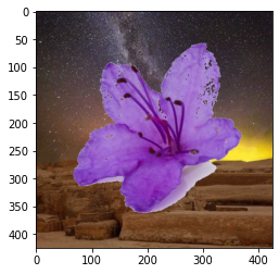
image = cv2.imread("assets/intro_opencv/petal.jpg", 1)

The second argument is a flag:

• 1 reads the image as a color image
• 0 reads the image as grayscale
• -1 reads the image unchanged

Example:

fg = cv2.imread("assets/intro_opencv/petal.jpg", 1)
fg = cv2.resize(fg, (425, 425))

print(fg.shape)

Output:

(425, 425, 3)

Display an Image with OpenCV

In a normal Python script, you can use:

cv2.imshow("image", fg)
cv2.waitKey(0)
cv2.destroyAllWindows()

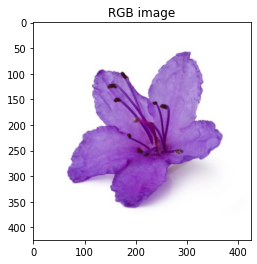
In Jupyter notebooks, Matplotlib is usually easier.

rgb_fg = cv2.cvtColor(fg, cv2.COLOR_BGR2RGB)

plt.imshow(rgb_fg)
plt.title("RGB image")
plt.axis("off")
plt.show()

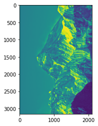
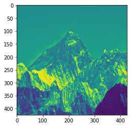
Display a Grayscale Image

img = cv2.imread("assets/intro_opencv/everest.jpg")

gray = cv2.cvtColor(img, cv2.COLOR_BGR2GRAY)

plt.imshow(gray, cmap="gray")
plt.axis("off")
plt.show()

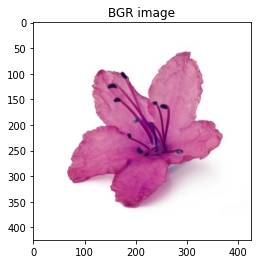
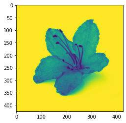
BGR vs RGB in OpenCV

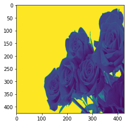
OpenCV reads images in BGR format. Matplotlib reads images in RGB format. If you directly show an OpenCV image with Matplotlib, the colors may look wrong.

plt.imshow(np.array(fg))
plt.title("BGR image shown with Matplotlib")
plt.axis("off")
plt.show()

Now convert BGR to RGB.

rgb_fg = cv2.cvtColor(fg, cv2.COLOR_BGR2RGB)

plt.imshow(rgb_fg)
plt.title("RGB image")
plt.axis("off")
plt.show()

Split Image Channels

We can access individual image channels using NumPy indexing.

red = np.zeros_like(rgb_fg, dtype=np.uint8)
red[:, :, 0] = rgb_fg[:, :, 0]

plt.imshow(red)
plt.axis("off")
plt.show()

green = np.zeros_like(rgb_fg, dtype=np.uint8)
green[:, :, 1] = rgb_fg[:, :, 1]

plt.imshow(green)
plt.axis("off")
plt.show()

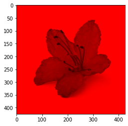
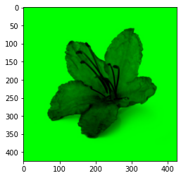
This helps us understand how each color channel contributes to the final image.

Image Transformations

Images can be transformed geometrically. Common transformations include:

• resizing
• rotation
• translation
• flipping
• cropping
• affine transformation
• perspective transformation

Resize an Image

resized = cv2.resize(fg, (425, 425))

Rotate an Image

gray_fg = cv2.cvtColor(fg, cv2.COLOR_BGR2GRAY)

rows, cols = gray_fg.shape

matrix = cv2.getRotationMatrix2D((cols / 2, rows / 2), 40, 1)
rotated = cv2.warpAffine(fg, matrix, (cols, rows))

plt.imshow(cv2.cvtColor(rotated, cv2.COLOR_BGR2RGB))
plt.axis("off")
plt.show()

The function cv2.getRotationMatrix2D creates a rotation matrix. Then cv2.warpAffine applies the transformation.

Image Masking

Image masking means selecting only a part of an image based on a condition. A mask is usually a binary image where:

• white pixels mean keep this part
• black pixels mean remove this part

Masking can be used for:

• background removal
• object extraction
• color-based selection
• image blending
• region of interest extraction

Basic Image Masking Example

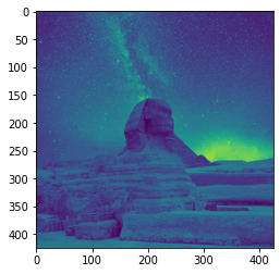
First, read the background image.

pyramid = cv2.imread("assets/intro_opencv/pyramid.jpg", 1)

print(pyramid.shape)

pyramid = cv2.resize(pyramid, (425, 425))

rgb_pyramid = cv2.cvtColor(pyramid, cv2.COLOR_BGR2RGB)

plt.imshow(rgb_pyramid)
plt.axis("off")
plt.show()

Convert both images to grayscale.

gray_fg = cv2.cvtColor(rgb_fg, cv2.COLOR_BGR2GRAY)
gray_pyramid = cv2.cvtColor(rgb_pyramid, cv2.COLOR_BGR2GRAY)

plt.imshow(gray_fg, cmap="gray")
plt.axis("off")
plt.show()

plt.imshow(gray_pyramid, cmap="gray")
plt.axis("off")
plt.show()

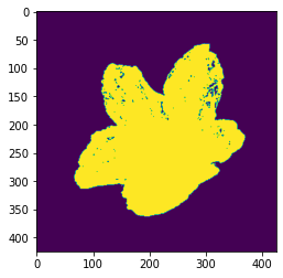
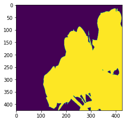
Create a mask.

lower_value = np.array([0, 0, 0])
higher_value = np.array([220, 220, 220])

mask = cv2.inRange(fg, lower_value, higher_value)

plt.imshow(mask, cmap="gray")
plt.axis("off")
plt.show()

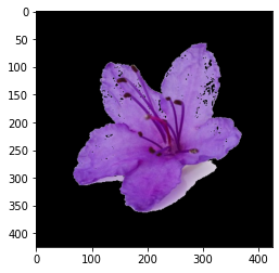
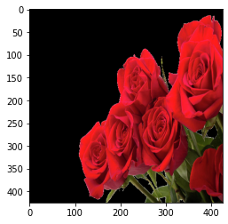
Apply the mask.

masked_img = rgb_fg.copy()
masked_img[mask != 255] = [0, 0, 0]

plt.imshow(masked_img)
plt.axis("off")
plt.show()

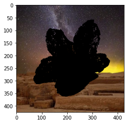
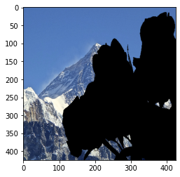
Now combine the foreground and background.

bg_copy = rgb_pyramid.copy()
bg_copy[mask == 255] = [0, 0, 0]

plt.imshow(bg_copy)
plt.axis("off")
plt.show()

final = bg_copy + masked_img

plt.imshow(final)
plt.axis("off")
plt.show()

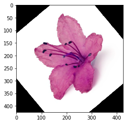
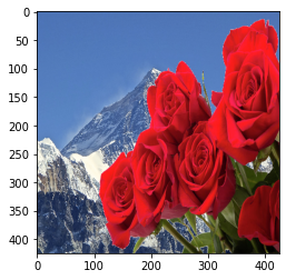
Full Masking Example

# Read foreground image
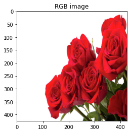
fg = cv2.imread("assets/intro_opencv/rose.jpg", 1)
fg = cv2.resize(fg, (425, 425))

# Convert BGR to RGB
rgb_fg = cv2.cvtColor(fg, cv2.COLOR_BGR2RGB)

plt.imshow(rgb_fg)
plt.title("RGB image")
plt.axis("off")
plt.show()

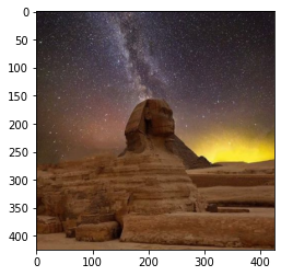
# Read background image
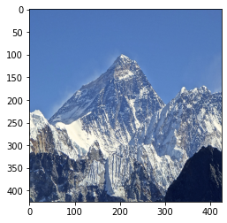
pyramid = cv2.imread("assets/intro_opencv/everest.jpg", 1)

print(pyramid.shape)

pyramid = cv2.resize(pyramid, (425, 425))

rgb_pyramid = cv2.cvtColor(pyramid, cv2.COLOR_BGR2RGB)

plt.imshow(rgb_pyramid)
plt.axis("off")
plt.show()

# Convert both images to grayscale
gray_fg = cv2.cvtColor(rgb_fg, cv2.COLOR_BGR2GRAY)
gray_pyramid = cv2.cvtColor(rgb_pyramid, cv2.COLOR_BGR2GRAY)

plt.imshow(gray_fg, cmap="gray")
plt.axis("off")
plt.show()

plt.imshow(gray_pyramid, cmap="gray")
plt.axis("off")
plt.show()

# Create mask
lower_value = np.array([0, 0, 0])
higher_value = np.array([220, 220, 255])

mask = cv2.inRange(fg, lower_value, higher_value)

plt.imshow(mask, cmap="gray")
plt.axis("off")
plt.show()

# Apply mask on foreground
masked_img = rgb_fg.copy()
masked_img[mask != 255] = [0, 0, 0]

plt.imshow(masked_img)
plt.axis("off")
plt.show()

# Remove masked area from background
bg_copy = rgb_pyramid.copy()
bg_copy[mask == 255] = [0, 0, 0]

plt.imshow(bg_copy)
plt.axis("off")
plt.show()

# Combine images
final = bg_copy + masked_img

plt.imshow(final)
plt.axis("off")
plt.show()

Exercise

Try using an image with a different background color and create a new mask for it.

Image Filtering

Image filtering is very important in computer vision. It is used for:

• blurring
• sharpening
• noise removal
• edge detection
• feature enhancement

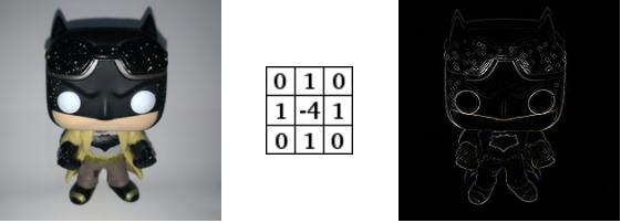
Filtering usually works through convolution. A small matrix called a kernel moves over the image. At each position, it multiplies nearby pixel values and creates a new output value.

Convolution in Image Processing

A convolution kernel can look like this:

kernel = np.array([
    [0, -1, 0],
    [-1, 4, -1],
    [0, -1, 0]
])

This type of kernel can highlight changes between neighboring pixels.

A high-pass filtering example:

A convolution process example:

High-Pass vs Low-Pass Filters

High-Pass Filters

High-pass filters are used for:

• sharpening
• enhancing features
• detecting edges
• highlighting sudden intensity changes

Example kernel:

np.array([
    [0, -1, 0],
    [-1, 4, -1],
    [0, -1, 0]
])

Low-Pass Filters

Low-pass filters are used for:

• smoothing
• blurring
• reducing noise
• removing small details

Examples include:

• mean blur
• box blur
• Gaussian blur
• median blur

Helper Function to Show Images

def show(img, title="image", cmap="gray"):
    plt.figure(figsize=(10, 10))
    plt.imshow(img, cmap=cmap)
    plt.title(title)
    plt.axis("off")
    plt.show()

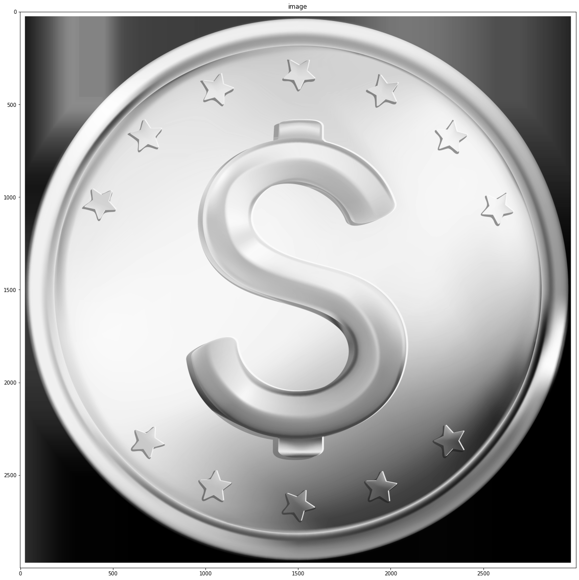
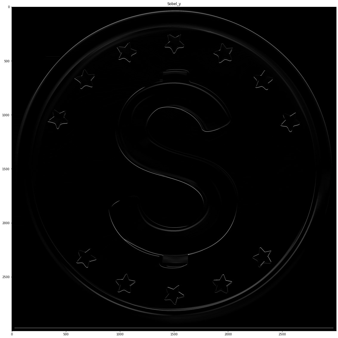
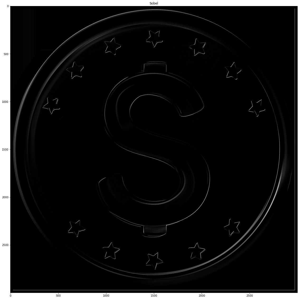
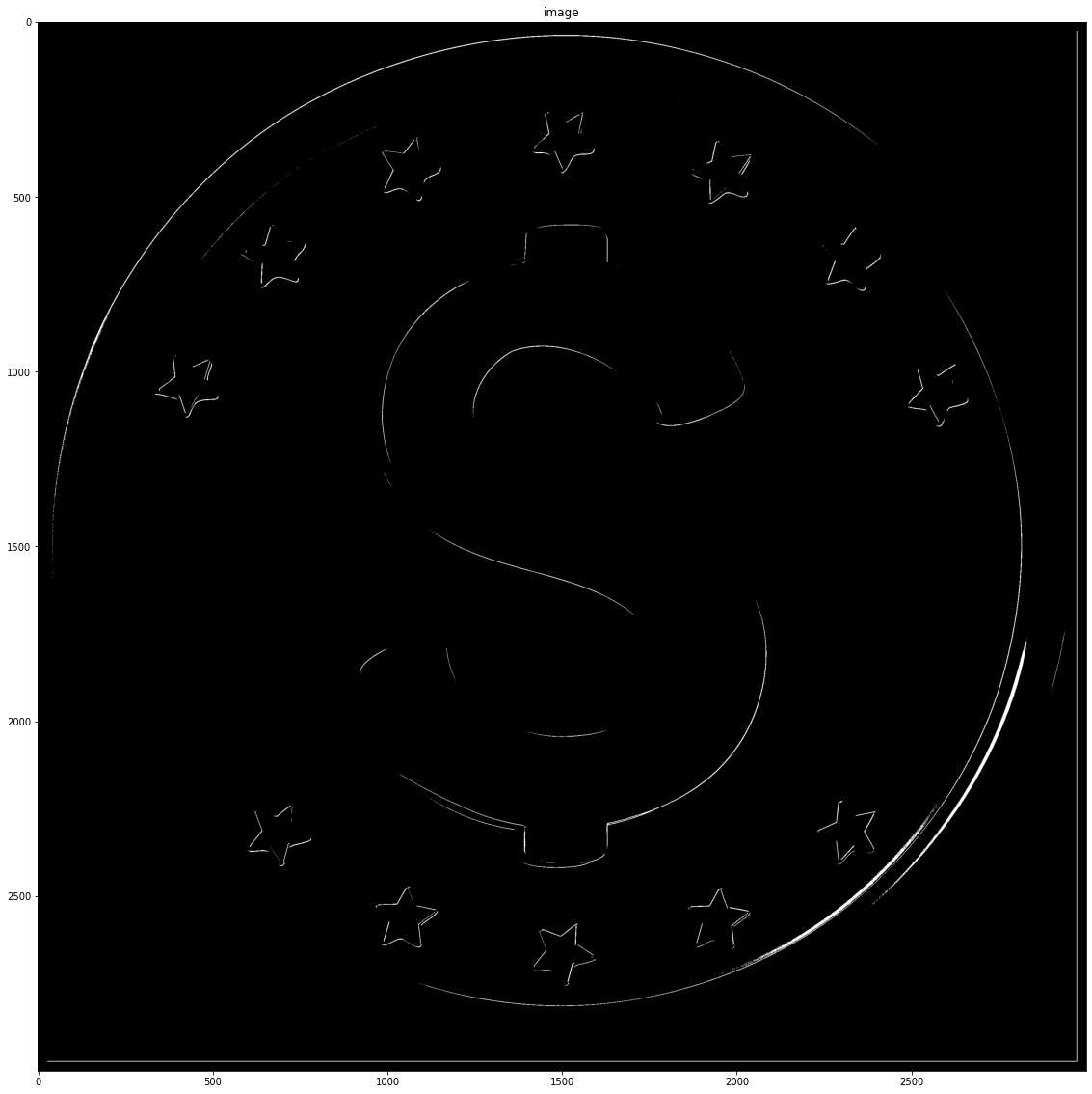
Sobel Edge Filtering

Sobel filters are used to detect changes in horizontal and vertical directions.

stripes = cv2.imread("assets/intro_opencv/coin.png", 0)

show(stripes)

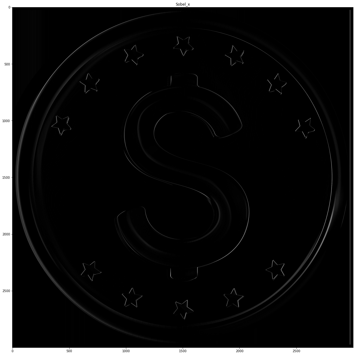
# Sobel x
kernel_x = np.array([
    [-1, 0, 1],
    [-2, 0, 2],
    [-1, 0, 1]
])

filtered_x = cv2.filter2D(stripes, -1, kernel_x)
show(filtered_x, "Sobel X")

# Sobel y
kernel_y = np.array([
    [-1, -2, -1],
    [0, 0, 0],
    [1, 2, 1]
])

filtered_y = cv2.filter2D(stripes, -1, kernel_y)
show(filtered_y, "Sobel Y")

kernel = kernel_x + kernel_y

filtered = cv2.filter2D(stripes, -1, kernel)
show(filtered, "Sobel")

Exercise

Try different high-pass and low-pass kernels and compare the output.

Low-Pass Filters and Blurring

Low-pass filters smooth the image. They are useful for reducing noise.

Common OpenCV blurring functions include:

cv2.blur(image, (5, 5))
cv2.GaussianBlur(image, (5, 5), 0)
cv2.medianBlur(image, 9)

Example:

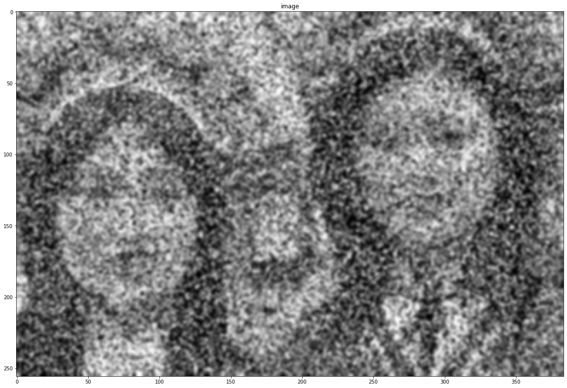
noise = cv2.imread("assets/intro_opencv/noise.png", 0)

show(noise)

kernel = np.ones([7, 7], dtype=np.float32) / 255

blurred = cv2.filter2D(noise, -1, kernel)
show(blurred, "Custom blur")

blurred = cv2.blur(noise, (5, 5))
show(blurred, "Average blur")

blurred = cv2.GaussianBlur(noise, (5, 5), 0)
show(blurred, "Gaussian blur")

blurred = cv2.medianBlur(noise, 9)
show(blurred, "Median blur")

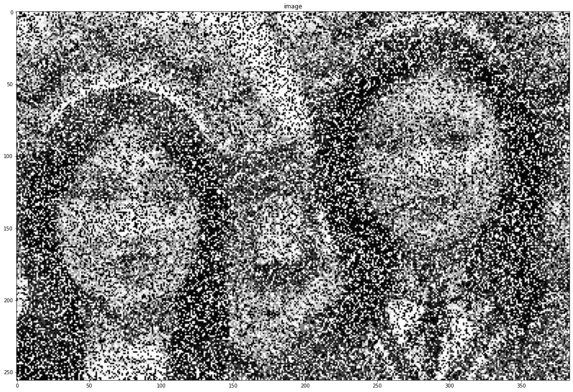
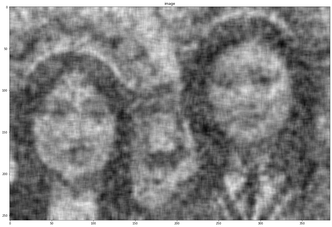
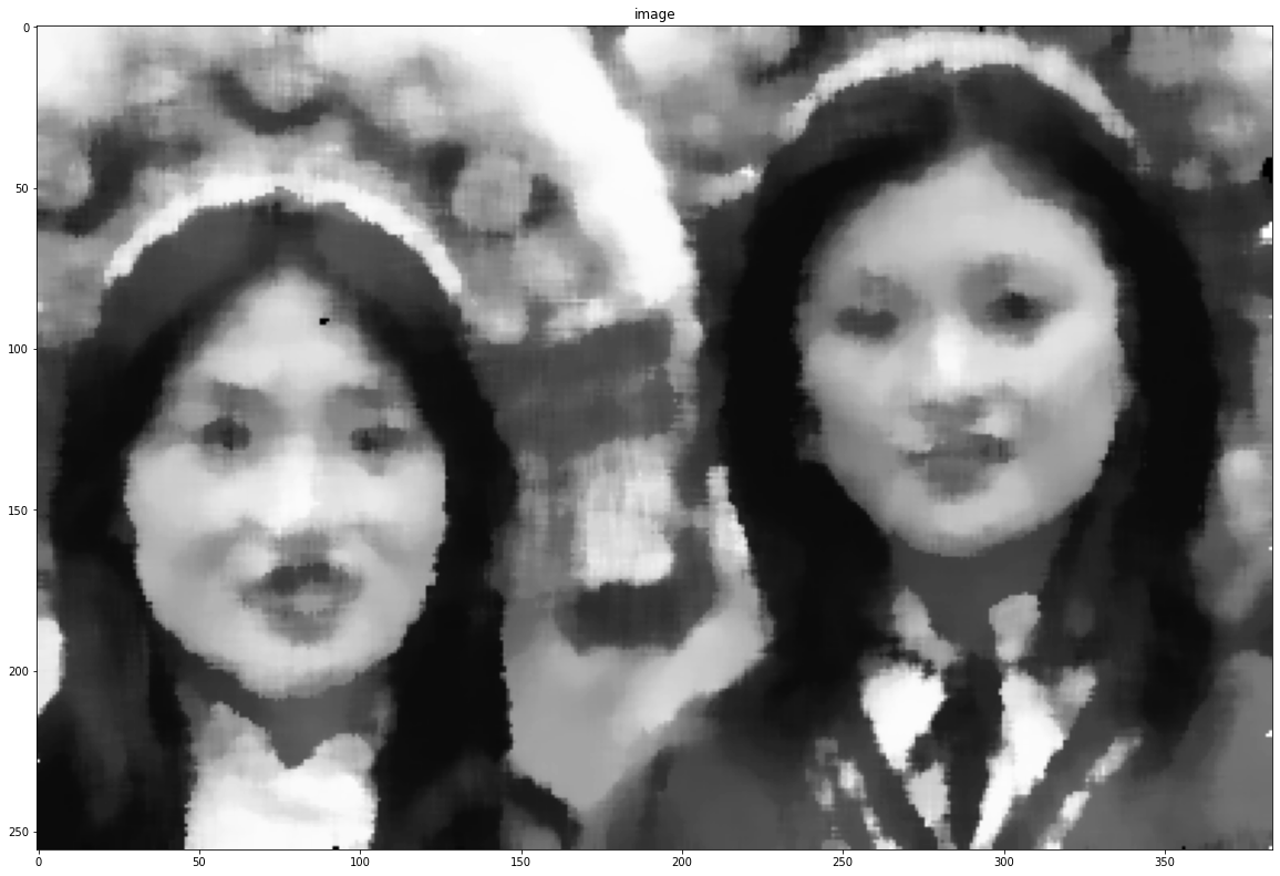
Median blur is useful for salt-and-pepper noise.

Image Thresholding

Thresholding converts an image into a binary or limited-value image based on pixel intensity.

retval, thresholded = cv2.threshold(
    filtered,
    100,
    200,
    cv2.THRESH_BINARY
)

show(thresholded)

Common thresholding methods include:

• binary thresholding
• inverse binary thresholding
• adaptive thresholding
• Otsu thresholding

Exercise

Try different threshold values and compare the results.

Canny Edge Detection

Canny edge detection is a popular edge detection method. It combines several steps:

1. noise reduction using Gaussian blur
2. gradient calculation using Sobel filters
3. non-maximum suppression
4. hysteresis thresholding

OpenCV implementation:

low = 10
high = 250

canny_img = cv2.Canny(stripes, low, high)

show(canny_img, "Canny")

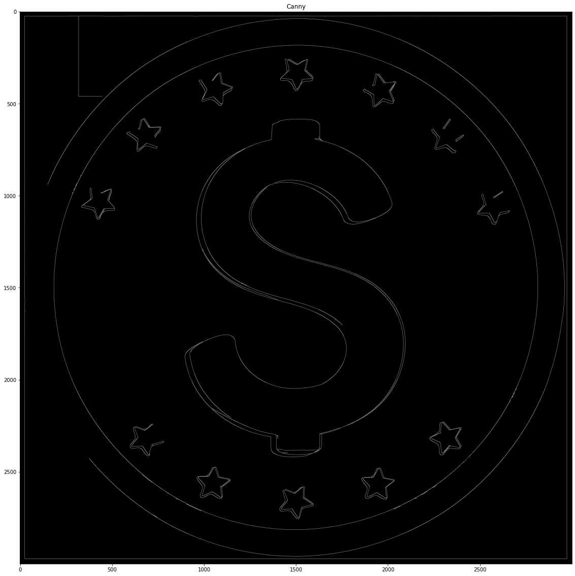
Canny edge detection is useful for object boundaries, shape extraction, and line detection.

Hough Transform

The Hough Transform is a popular method for detecting lines and shapes.

It can detect:

• lines
• circles
• other geometric shapes with proper equations

First, read the image and apply Canny edge detection.

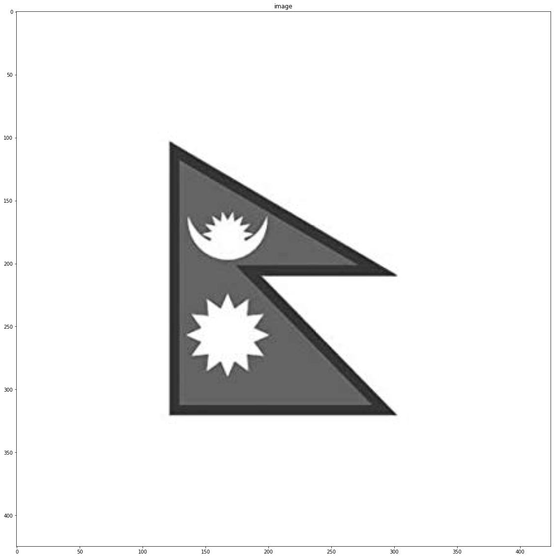
img = cv2.imread("assets/intro_opencv/flag.jpg", 0)

show(img)

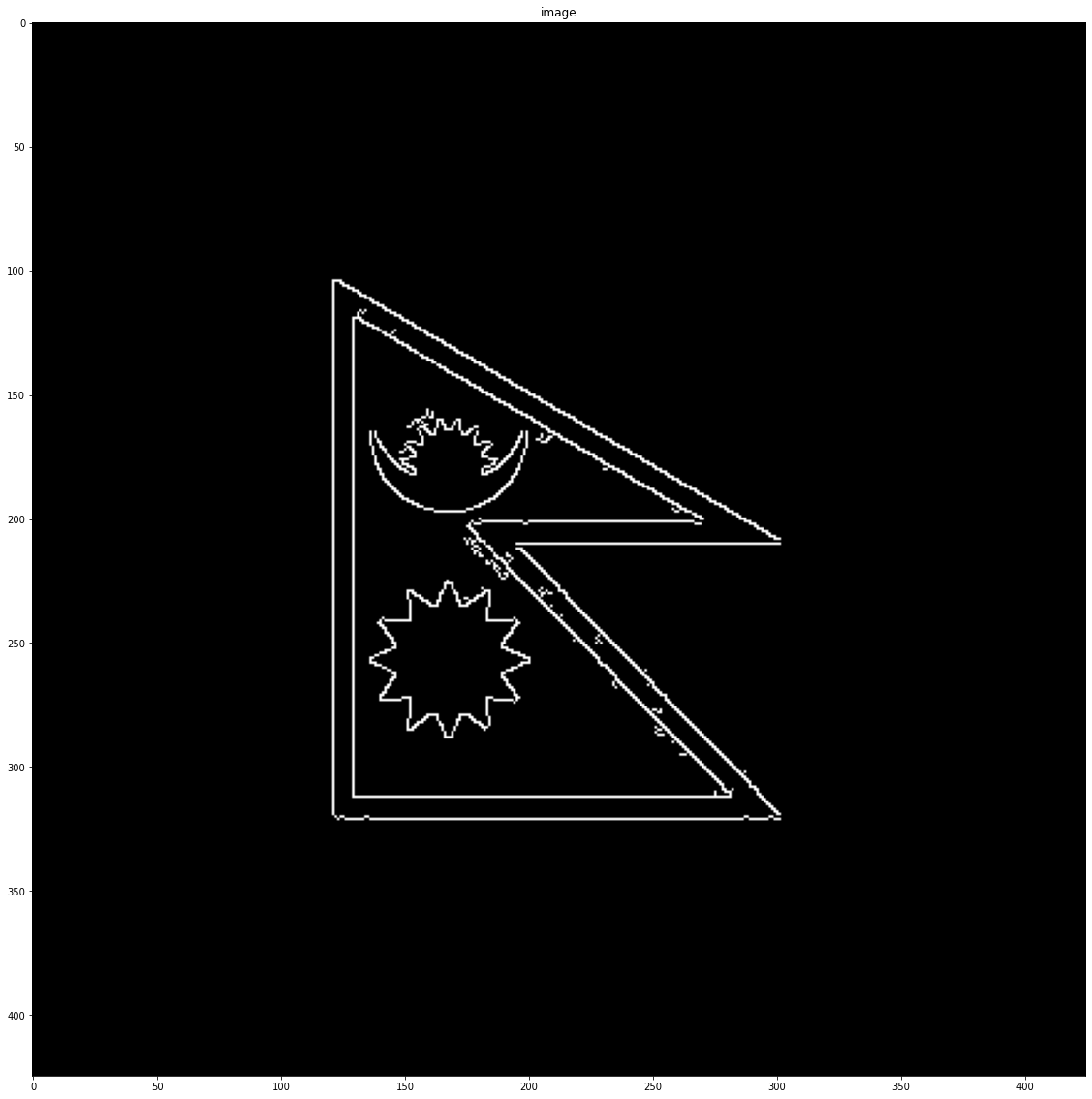
canny_img = cv2.Canny(img, low, high)

show(canny_img)

Hough Transform for Line Detection

rho = 1
theta = np.pi / 180
threshold = 60
max_line_length = 50
max_line_gap = 50

lines = cv2.HoughLinesP(
    canny_img,
    rho,
    theta,
    threshold,
    np.array([]),
    max_line_length,
    max_line_gap
)

line_img = img.copy()

for line in lines:
    for x1, y1, x2, y2 in line:
        cv2.line(line_img, (x1, y1), (x2, y2), (0, 255, 0), 2)

show(line_img)

Hough Transform is useful when we want to detect lines in roads, documents, lanes, borders, or geometric objects.

Haar Cascade for Face Detection

Haar cascade is a classical object detection method. It uses pre-trained XML files to detect objects such as faces and eyes.

OpenCV includes some Haar cascade XML files.

img = cv2.imread("assets/intro_opencv/xmen.jpg", 1)
gray = cv2.cvtColor(img, cv2.COLOR_BGR2GRAY)

cascade_dir = "C:/ProgramData/Anaconda3/Lib/site-packages/cv2/data/"

face_cascade = cv2.CascadeClassifier(
    cascade_dir + "haarcascade_frontalface_default.xml"
)

eye_cascade = cv2.CascadeClassifier(
    cascade_dir + "haarcascade_eye.xml"
)

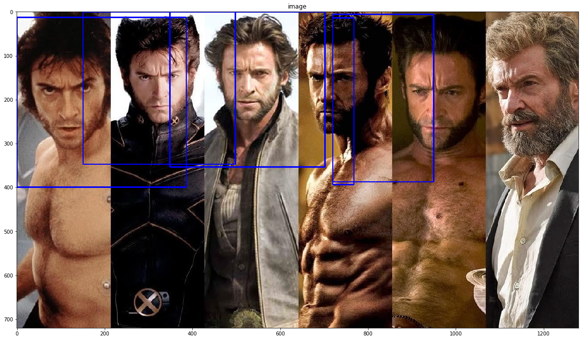
faces = face_cascade.detectMultiScale(gray, 1.3, 5)

padding = 100
height, width = gray.shape

for (x, y, w, h) in faces:
    y = np.clip(y - padding, 0, y)
    x = np.clip(x - padding, 0, x)
    w = np.clip(w + 2 * padding, 0, width - x)
    h = np.clip(h + 2 * padding, 0, height - y)

    img = cv2.rectangle(img, (x, y), (x + w, y + h), (255, 0, 0), 2)

show(cv2.cvtColor(img, cv2.COLOR_BGR2RGBA))

Exercise

Try other Haar cascade XML files and detect eyes, smiles, or full bodies.

Contours in OpenCV

Contours are curves that join continuous points along an object boundary. They are useful for shape detection and object boundary extraction.

For example, if we want to extract the boundary of a bottle, the contour will follow the bottle edges.

img = cv2.imread("assets/intro_opencv/flag.jpg")
img_gray = cv2.cvtColor(img, cv2.COLOR_BGR2GRAY)

_, thresh = cv2.threshold(
    img_gray,
    0,
    255,
    cv2.THRESH_BINARY + cv2.THRESH_OTSU
)

contours, hierarchy = cv2.findContours(
    thresh,
    cv2.RETR_TREE,
    cv2.CHAIN_APPROX_SIMPLE
)

cnt = contours[0]

hull = cv2.convexHull(cnt, returnPoints=False)

defects = cv2.convexityDefects(cnt, hull)

for i in range(defects.shape[0]):
    s, e, f, d = defects[i, 0]

    start = tuple(cnt[s][0])
    end = tuple(cnt[e][0])
    far = tuple(cnt[f][0])

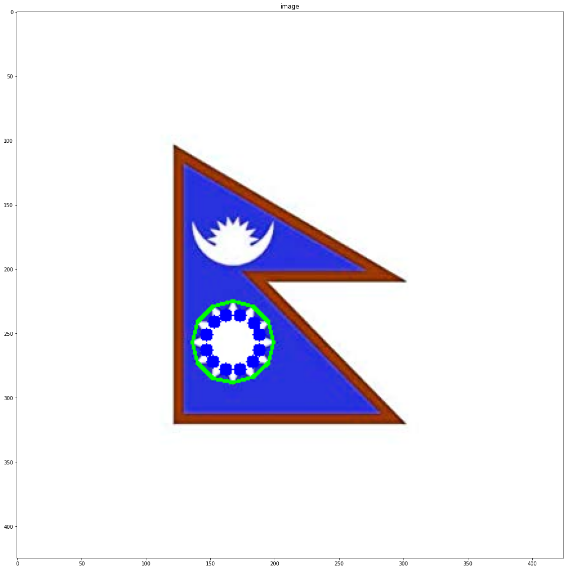
    cv2.line(img, start, end, [0, 255, 0], 2)
    cv2.circle(img, far, 5, [0, 0, 255], -1)

show(img)

Contours are useful for:

• shape detection
• object counting
• document boundary extraction
• hand gesture detection
• measuring object area
• finding object outlines

Color Tracking in OpenCV

Color tracking is easier in HSV color space.

HSV stands for:

• Hue
• Saturation
• Value

In OpenCV:

• Hue range is usually 0 to 179
• Saturation range is 0 to 255
• Value range is 0 to 255

The example below tracks white color using a webcam.

import cv2
import numpy as np

cap = cv2.VideoCapture(0)

while True:
    ret, frame = cap.read()

    if not ret:
        break

    hsv = cv2.cvtColor(frame, cv2.COLOR_BGR2HSV)

    lower_white = np.array([0, 0, 0], dtype=np.uint8)
    upper_white = np.array([20, 20, 255], dtype=np.uint8)

    mask = cv2.inRange(hsv, lower_white, upper_white)

    result = cv2.bitwise_and(frame, frame, mask=mask)

    cv2.imshow("frame", frame)
    cv2.imshow("mask", mask)
    cv2.imshow("result", result)

    key = cv2.waitKey(5) & 0xFF

    if key == 27:
        break

cap.release()
cv2.destroyAllWindows()

This can be modified to track other colors by changing the lower and upper HSV ranges.

Introduction to YOLO with OpenCV DNN

YOLO means You Only Look Once. It is an object detection method that can detect multiple objects in an image.

The original YOLO paper is available here:

• YOLO paper

YOLO models trained on COCO can detect common object classes such as person, car, dog, bottle, chair, and many more.

YOLO Setup

For classic YOLOv3 with OpenCV DNN, you need:

• YOLOv3 weights
• YOLOv3 configuration file
• COCO class labels

Original resources:

• Weights: https://pjreddie.com/media/files/yolov3.weights
• Config: https://github.com/pjreddie/darknet/blob/master/cfg/yolov3.cfg
• Labels: https://github.com/pjreddie/darknet/blob/master/data/coco.names

Load YOLO with OpenCV

net = cv2.dnn.readNet("yolov3.weights", "yolov3.cfg")

layer_names = net.getLayerNames()

output_layers = [
    layer_names[i - 1]
    for i in net.getUnconnectedOutLayers().flatten()
]

In older OpenCV versions, getUnconnectedOutLayers() may return a different shape, so some examples use i[0] - 1.

Create a Blob and Run YOLO

blob = cv2.dnn.blobFromImage(
    img,
    0.00392,
    (416, 416),
    (0, 0, 0),
    True,
    crop=False
)

net.setInput(blob)

outs = net.forward(output_layers)

The output contains:

• bounding box center coordinates
• width and height
• class scores
• confidence values

Usually, we apply Non-Maximum Suppression, or NMS, to remove duplicate boxes around the same object.

Common OpenCV Beginner Mistakes

Here are some common mistakes to avoid:

• forgetting that OpenCV reads images as BGR
• showing BGR images directly with Matplotlib
• using cv2.imshow inside notebooks
• using wrong image paths
• not checking whether cv2.imread returned None
• mixing grayscale and color images without checking shape
• using too high or too low threshold values
• applying filters without understanding the kernel
• not converting to HSV before color tracking
• forgetting to release webcam with cap.release()

A good habit is to always check:

if img is None:
    raise FileNotFoundError("Image path is wrong or image could not be loaded.")

Final Thoughts

In this post, we covered the basics of OpenCV image processing in Python. We learned how images are represented as arrays, how to read and display images, how to work with color channels, and how to apply transformations, masks, filters, thresholding, edge detection, Hough Transform, contours, Haar cascade face detection, YOLO, and color tracking.

OpenCV is a large library, and this post only gives an introduction. The best way to learn OpenCV is to try small projects, change parameters, and observe how the output changes.