CNN with Keras: Beginner Guide to Convolutional Neural Networks for Image Classification

11 minute read

A Convolutional Neural Network, or CNN, is one of the most important deep learning architectures for image-related tasks. CNNs are widely used for image classification, object detection, segmentation, face recognition, medical imaging, satellite image analysis, and many other computer vision problems.

In this blog, we will learn the basics of CNN with Keras. Keras makes it easy to build neural networks layer by layer without writing every mathematical operation from scratch.

I originally wrote this notebook in 2019 when I was learning CNNs. I have now rewritten it as a cleaner beginner-friendly tutorial with modern Keras-style code and better explanations.

Note: Some images used in the original version of this post were collected from the internet while I was learning. Full credit belongs to the original image authors.

What This Tutorial Covers

In this tutorial, we will cover:

why Keras is useful
what a CNN is
why CNNs work well for images
basic CNN terms
convolution layers
filters and kernels
stride and padding
feature maps
max pooling
dropout
flatten and dense layers
a simple CNN architecture
loading image data with Keras
data augmentation
compiling and training a CNN
overfitting and how to reduce it
common beginner mistakes

Why Keras?

Keras is a high-level deep learning API. It lets us build neural networks by stacking layers together.

Keras is beginner-friendly because:

it is easy to read
it is easy to build models quickly
it hides many low-level details
it supports common deep learning layers
it has tools for preprocessing images
it works well with TensorFlow
it supports fast experimentation

In older code, we often wrote imports like this:

from keras.models import Sequential
from keras.layers import Conv2D, MaxPooling2D, Flatten, Dense, Dropout

In modern TensorFlow projects, you will often see:

import tensorflow as tf

from tensorflow import keras
from tensorflow.keras import layers

Both styles may work depending on your environment, but the TensorFlow Keras style is common in many tutorials.

Install TensorFlow and Keras

If TensorFlow is not installed, you can install it with:

pip install tensorflow

Then import it:

import tensorflow as tf

from tensorflow import keras
from tensorflow.keras import layers

print(tf.__version__)

If you are using standalone Keras 3, you may also see:

pip install keras

For beginners, using TensorFlow with Keras is usually the easiest starting point.

What Is a CNN?

A Convolutional Neural Network is a neural network that uses convolution operations to learn patterns from data.

CNNs are mostly used for images, but they can also be used for other structured data such as time series, audio, and text.

In simple words:

A CNN learns small visual patterns first, then combines them into larger and more meaningful patterns.

For example, in an image classifier:

early layers may learn edges and corners
middle layers may learn textures and shapes
deeper layers may learn object parts
final layers classify the image

Why CNNs Are Useful for Images

A normal fully connected neural network treats every pixel as a separate input. For images, this can create too many parameters.

CNNs are better for images because:

they use small filters instead of connecting every pixel to every neuron
the same filter is reused across the whole image
they preserve spatial structure
they can learn local patterns such as edges and textures
they reduce the number of trainable parameters
they work well with image data

This is why CNNs are commonly used in computer vision.

Basic CNN Terms

Before building a CNN with Keras, we need to understand some basic terms.

Image Channels

A grayscale image has one channel.

An RGB image has three channels:

Red
Green
Blue

For example, an RGB image of size 224 x 224 has shape:

(224, 224, 3)

Filter or Kernel

A filter is a small matrix that slides over an image. It is used to detect patterns.

For example, a 3 x 3 filter looks at a small region of the image at a time.

Feature Map

When a filter is applied to an image, it produces a new output called a feature map.

Each filter creates one feature map.

Stride

Stride controls how many pixels the filter moves at a time.

stride 1 means the filter moves one pixel at a time
stride 2 means the filter moves two pixels at a time

Larger stride reduces the output size.

Padding

Padding means adding extra pixels around the border of an image.

Padding helps control the output size and allows filters to work better near image edges.

Common padding types are:

valid: no padding
same: output size is kept similar to input size

CNN Visualization

Here is a simple visualization of a CNN idea:

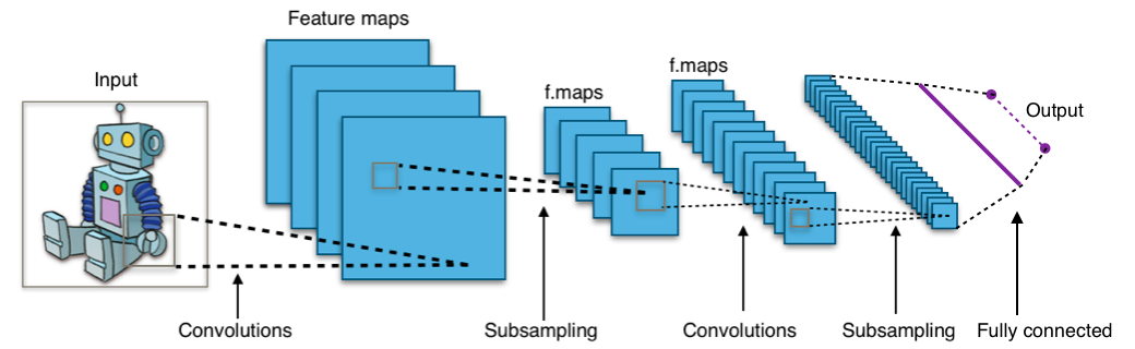
CNN layers manipulate images using kernels and learn useful patterns from them.

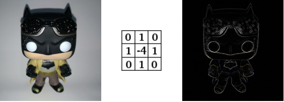
What Happens Inside a Convolution Layer?

A convolution layer applies filters over an image. Each filter slides over the image and performs element-wise multiplication and summation.

For a grayscale image, convolution can be visualized like this:

Inside a grayscale image convolution

For an RGB image, the convolution happens across multiple channels.

Inside an RGB image convolution

Padding adds extra pixels around the image border.

Padding of pixels

Common Layers in a CNN

A normal CNN often includes:

input layer
convolutional layers
activation functions
pooling layers
dropout layers
flatten layer
dense layers
output layer

Let’s understand each one.

Convolutional Layer

The convolutional layer is the main layer in a CNN.

In Keras, we usually use Conv2D.

layers.Conv2D(
    filters=32,
    kernel_size=(3, 3),
    activation="relu",
    padding="same"
)

Important arguments are:

filters: number of filters to learn
kernel_size: size of the filter
activation: activation function
padding: how borders are handled
strides: how far the filter moves

Example:

layers.Conv2D(32, (3, 3), activation="relu", padding="same")

This creates 32 filters of size 3 x 3.

ReLU Activation

CNNs commonly use the ReLU activation function.

activation="relu"

ReLU stands for Rectified Linear Unit. It keeps positive values and converts negative values to zero.

It helps the network learn non-linear patterns.

Max Pooling Layer

The MaxPooling2D layer reduces the spatial size of feature maps.

It keeps the maximum value from a small window.

For example, a 2 x 2 max pooling operation reduces the height and width by half.

Pooling window movement

Max pooling example

In Keras:

layers.MaxPooling2D(pool_size=(2, 2))

Max pooling helps:

reduce computation
reduce feature map size
make features more robust
control overfitting

Dropout Layer

Dropout is used to reduce overfitting.

During training, dropout randomly sets some input units to zero. This prevents the model from depending too much on specific neurons.

layers.Dropout(0.5)

A dropout value of 0.5 means 50 percent of the units are randomly dropped during training.

Dropout is active during training, not during normal prediction.

Flatten Layer

A convolution layer outputs a 3D feature map.

Dense layers need a 1D vector.

The Flatten layer converts the feature map into a one-dimensional vector.

layers.Flatten()

For example:

(7, 7, 64) -> 3136

Dense Layer

A dense layer is a fully connected layer.

In CNNs, dense layers are usually used near the end for classification.

layers.Dense(128, activation="relu")

For binary classification, the output layer can be:

layers.Dense(1, activation="sigmoid")

For multi-class classification, the output layer can be:

layers.Dense(num_classes, activation="softmax")

A Simple CNN with Keras

Here is a simple CNN model for image classification.

import tensorflow as tf

from tensorflow import keras
from tensorflow.keras import layers


num_classes = 2
image_size = (224, 224)

model = keras.Sequential([
    layers.Input(shape=(image_size[0], image_size[1], 3)),

    layers.Rescaling(1.0 / 255),

    layers.Conv2D(32, (3, 3), activation="relu", padding="same"),
    layers.MaxPooling2D((2, 2)),

    layers.Conv2D(64, (3, 3), activation="relu", padding="same"),
    layers.MaxPooling2D((2, 2)),

    layers.Conv2D(128, (3, 3), activation="relu", padding="same"),
    layers.MaxPooling2D((2, 2)),

    layers.Flatten(),

    layers.Dense(128, activation="relu"),
    layers.Dropout(0.5),

    layers.Dense(num_classes, activation="softmax")
])

model.summary()

This model has:

input layer
rescaling layer
three convolution blocks
flatten layer
dense layer
dropout layer
output layer

Compile the CNN Model

Before training, we compile the model.

model.compile(
    optimizer="adam",
    loss="sparse_categorical_crossentropy",
    metrics=["accuracy"]
)

Here:

optimizer="adam" controls how the model updates weights
loss="sparse_categorical_crossentropy" is used for integer class labels
metrics=["accuracy"] tracks classification accuracy

For binary classification with one output neuron and sigmoid activation, you can use:

model.compile(
    optimizer="adam",
    loss="binary_crossentropy",
    metrics=["accuracy"]
)

Loading Image Data with Keras

Keras can load image data directly from folders using image_dataset_from_directory.

A common folder structure is:

dataset/
    train/
        cats/
        dogs/
    validation/
        cats/
        dogs/

Load training data:

train_ds = keras.utils.image_dataset_from_directory(
    "dataset/train",
    image_size=(224, 224),
    batch_size=32
)

Load validation data:

val_ds = keras.utils.image_dataset_from_directory(
    "dataset/validation",
    image_size=(224, 224),
    batch_size=32
)

Keras automatically uses the folder names as labels.

Improve Dataset Performance

We can improve data loading performance using caching and prefetching.

AUTOTUNE = tf.data.AUTOTUNE

train_ds = train_ds.cache().shuffle(1000).prefetch(buffer_size=AUTOTUNE)
val_ds = val_ds.cache().prefetch(buffer_size=AUTOTUNE)

This helps the GPU or CPU receive data faster during training.

Data Augmentation

Data augmentation creates random variations of images during training.

It can help reduce overfitting.

data_augmentation = keras.Sequential([
    layers.RandomFlip("horizontal"),
    layers.RandomRotation(0.1),
    layers.RandomZoom(0.1),
])

Add it to the model:

model = keras.Sequential([
    layers.Input(shape=(224, 224, 3)),
    data_augmentation,
    layers.Rescaling(1.0 / 255),

    layers.Conv2D(32, (3, 3), activation="relu", padding="same"),
    layers.MaxPooling2D((2, 2)),

    layers.Conv2D(64, (3, 3), activation="relu", padding="same"),
    layers.MaxPooling2D((2, 2)),

    layers.Conv2D(128, (3, 3), activation="relu", padding="same"),
    layers.MaxPooling2D((2, 2)),

    layers.Flatten(),

    layers.Dense(128, activation="relu"),
    layers.Dropout(0.5),

    layers.Dense(num_classes, activation="softmax")
])

Common augmentation methods include:

random flip
random rotation
random zoom
random contrast
random translation

Train the CNN Model

history = model.fit(
    train_ds,
    validation_data=val_ds,
    epochs=10
)

During training, Keras shows metrics such as:

training loss
training accuracy
validation loss
validation accuracy

Plot Training History

import matplotlib.pyplot as plt

plt.plot(history.history["accuracy"], label="train accuracy")
plt.plot(history.history["val_accuracy"], label="validation accuracy")

plt.xlabel("Epoch")
plt.ylabel("Accuracy")
plt.legend()
plt.show()

Plot loss:

plt.plot(history.history["loss"], label="train loss")
plt.plot(history.history["val_loss"], label="validation loss")

plt.xlabel("Epoch")
plt.ylabel("Loss")
plt.legend()
plt.show()

These plots help us detect overfitting and underfitting.

Use Callbacks

Callbacks let us control training.

Two useful callbacks are:

EarlyStopping
ModelCheckpoint

callbacks = [
    keras.callbacks.EarlyStopping(
        monitor="val_loss",
        patience=3,
        restore_best_weights=True
    ),
    keras.callbacks.ModelCheckpoint(
        "best_cnn_model.keras",
        monitor="val_loss",
        save_best_only=True
    )
]

Use callbacks during training:

history = model.fit(
    train_ds,
    validation_data=val_ds,
    epochs=30,
    callbacks=callbacks
)

EarlyStopping stops training when validation loss stops improving.

ModelCheckpoint saves the best model.

Make Predictions

After training, we can use the model for prediction.

import numpy as np

image_path = "test_image.jpg"

img = keras.utils.load_img(
    image_path,
    target_size=(224, 224)
)

img_array = keras.utils.img_to_array(img)
img_array = np.expand_dims(img_array, axis=0)

predictions = model.predict(img_array)

predicted_class = np.argmax(predictions[0])

print(predicted_class)
print(predictions)

If you know the class names:

class_names = train_ds.class_names

print(class_names[predicted_class])

Save and Load a Keras Model

Save the model:

model.save("cnn_model.keras")

Load it later:

loaded_model = keras.models.load_model("cnn_model.keras")

This is useful when you want to deploy or reuse the trained model.

Overfitting in CNNs

Overfitting happens when a model performs very well on training data but poorly on validation or test data.

For example:

Training accuracy: 98%
Validation accuracy: 62%

This means the model may be memorizing the training images instead of learning general patterns.

Why Overfitting Happens

Overfitting can happen because:

the model is too complex
the dataset is too small
training runs for too many epochs
images are not diverse enough
there is no data augmentation
there is no regularization
train and validation data are not properly split

How to Reduce Overfitting

Some common solutions are:

use more training data
use data augmentation
add dropout
reduce model size
use early stopping
use regularization
use transfer learning
normalize image pixels
check train and validation split carefully

In Keras, dropout can be added like this:

layers.Dropout(0.5)

Early stopping can be added like this:

keras.callbacks.EarlyStopping(
    monitor="val_loss",
    patience=3,
    restore_best_weights=True
)

Transfer Learning

For many real-world image projects, training a CNN from scratch is not the best starting point.

Instead, we can use a pre-trained model such as:

MobileNetV2
EfficientNet
ResNet
VGG16

These models are already trained on large image datasets. We can reuse them and train only the final classification layers for our own task.

Example with MobileNetV2:

base_model = keras.applications.MobileNetV2(
    input_shape=(224, 224, 3),
    include_top=False,
    weights="imagenet"
)

base_model.trainable = False

model = keras.Sequential([
    layers.Input(shape=(224, 224, 3)),
    layers.Rescaling(1.0 / 255),

    base_model,

    layers.GlobalAveragePooling2D(),
    layers.Dropout(0.3),

    layers.Dense(num_classes, activation="softmax")
])

Transfer learning is often faster and more accurate than training a small CNN from scratch.

CNN from Scratch vs Transfer Learning

Approach	Best For	Pros	Cons
CNN from scratch	Learning, simple datasets	Easy to understand	Needs more data
Transfer learning	Real projects	Usually better accuracy	Slightly more complex
Fine-tuning	Advanced projects	Can improve performance	Needs careful training

For beginners, it is good to first build a CNN from scratch to understand the idea. Then try transfer learning.

Common Beginner Mistakes

Here are common mistakes when learning CNN with Keras:

forgetting to rescale image pixels
using wrong input shape
using softmax with one output neuron
using sigmoid with many classes
using the wrong loss function
training too long without checking validation loss
not using validation data
using too large a model for a small dataset
forgetting data augmentation
mixing RGB and BGR images
not checking class labels
assuming high training accuracy means a good model

Which Loss Function Should You Use?

Problem Type	Output Layer	Loss Function
Binary classification	`Dense(1, activation="sigmoid")`	`binary_crossentropy`
Multi-class with integer labels	`Dense(num_classes, activation="softmax")`	`sparse_categorical_crossentropy`
Multi-class with one-hot labels	`Dense(num_classes, activation="softmax")`	`categorical_crossentropy`

Choosing the right output layer and loss function is very important.

Full CNN Example

Here is a complete beginner-friendly CNN example.

import tensorflow as tf

from tensorflow import keras
from tensorflow.keras import layers


image_size = (224, 224)
batch_size = 32
num_classes = 2

train_ds = keras.utils.image_dataset_from_directory(
    "dataset/train",
    image_size=image_size,
    batch_size=batch_size
)

val_ds = keras.utils.image_dataset_from_directory(
    "dataset/validation",
    image_size=image_size,
    batch_size=batch_size
)

AUTOTUNE = tf.data.AUTOTUNE

train_ds = train_ds.cache().shuffle(1000).prefetch(buffer_size=AUTOTUNE)
val_ds = val_ds.cache().prefetch(buffer_size=AUTOTUNE)

data_augmentation = keras.Sequential([
    layers.RandomFlip("horizontal"),
    layers.RandomRotation(0.1),
    layers.RandomZoom(0.1),
])

model = keras.Sequential([
    layers.Input(shape=(224, 224, 3)),
    data_augmentation,
    layers.Rescaling(1.0 / 255),

    layers.Conv2D(32, (3, 3), activation="relu", padding="same"),
    layers.MaxPooling2D((2, 2)),

    layers.Conv2D(64, (3, 3), activation="relu", padding="same"),
    layers.MaxPooling2D((2, 2)),

    layers.Conv2D(128, (3, 3), activation="relu", padding="same"),
    layers.MaxPooling2D((2, 2)),

    layers.Flatten(),

    layers.Dense(128, activation="relu"),
    layers.Dropout(0.5),

    layers.Dense(num_classes, activation="softmax")
])

model.compile(
    optimizer="adam",
    loss="sparse_categorical_crossentropy",
    metrics=["accuracy"]
)

callbacks = [
    keras.callbacks.EarlyStopping(
        monitor="val_loss",
        patience=3,
        restore_best_weights=True
    )
]

history = model.fit(
    train_ds,
    validation_data=val_ds,
    epochs=20,
    callbacks=callbacks
)

model.save("cnn_model.keras")

Final Thoughts

In this blog, we learned the basics of CNN with Keras. We discussed convolution layers, filters, feature maps, stride, padding, max pooling, dropout, flatten layers, dense layers, image data loading, augmentation, training, and overfitting.

CNNs are one of the most important tools in computer vision. Keras makes them much easier to build and experiment with. The best way to learn is to start with a small image classification dataset, train a simple CNN, inspect the training curves, and then try transfer learning with a pre-trained model.

Twitter Facebook LinkedIn

Quassarian Viper