Making Fractal Shapes with Python: Cantor Set, Koch Curve, and Sierpinski Triangle

Fractals are never-ending patterns that repeat at different scales. They are often seen in nature, mathematics, art, and computer graphics. A fractal shape can look complex, but many fractals are created by repeating a simple rule again and again.

Fractals can be found in many natural structures, such as:

• fern leaves
• tree branches
• clouds
• coastlines
• snowflakes
• water ripples
• lightning patterns
• blood vessels
• neural structures

Fractals are different from classical geometry. In classical geometry, we often work with simple shapes such as lines, circles, triangles, and rectangles. In fractal geometry, we build complex shapes from repeated rules, recursion, and self-similar patterns.

In this tutorial, we will create fractal shapes with Python using NumPy and Matplotlib.

We will cover:

• what fractals are
• Middle Third Cantor Set
• section formula for dividing a line
• Von Koch Curve
• Sierpinski Triangle
• recursive and iterative fractal generation
• plotting fractals with Matplotlib
• beginner exercises

What Is a Fractal?

A fractal is a pattern that repeats itself at different levels of scale.

One important idea in fractal geometry is self-similarity. This means that a small part of the shape looks similar to the whole shape.

For example, a fern leaf has smaller leaf parts that look similar to the full fern. A tree branch also looks like a smaller version of the whole tree structure.

Fractals are usually created by repeating a simple rule many times.

Why Use Python for Fractals?

Python is a good language for drawing fractals because it has simple tools for mathematics and plotting.

In this post, we will use:

import matplotlib.pyplot as plt
import numpy as np

We use:

• NumPy for handling points and arrays
• Matplotlib for plotting lines and shapes

Middle Third Cantor Set

While writing the original version of this blog, I was reading the book Fractal Geometry: Mathematical Foundations and Applications. So, I started with a classical fractal example from that book.

FRACTAL GEOMETRY Mathematical Foundations and Applications: Page XVIII

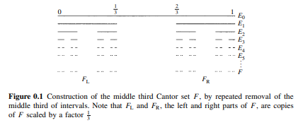
The Middle Third Cantor Set is one of the simplest fractals.

The construction steps are:

1. Start with a straight line.
2. Divide the line into three equal parts.
3. Remove the middle third.
4. Now there are two smaller line segments.
5. Repeat the same process for every remaining segment.
6. Continue until the desired number of steps.

After every step, the number of segments doubles, and each segment becomes smaller.

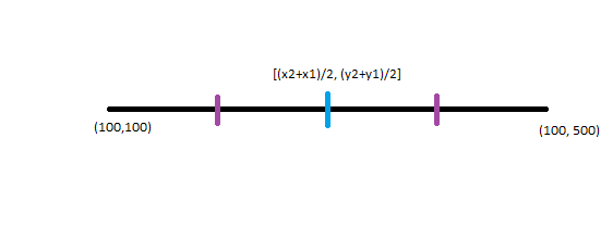
Section Formula

To create the Cantor Set, we need to divide a line into three equal parts. For this, we can use the section formula.

Suppose a line goes from:

(x1, y1) to (x2, y2)

To divide the line into three equal parts, we need two points between the endpoints.

The first point is:

\[x_3 = \frac{x_1 n + x_2 m}{m+n}\] \[y_3 = \frac{y_1 n + y_2 m}{m+n}\]

The second point is:

\[x_4 = \frac{x_1 m + x_2 n}{m+n}\] \[y_4 = \frac{y_1 m + y_2 n}{m+n}\]

For dividing a line into three equal parts, we can use:

m = 1
n = 2

This gives the two points that cut the line into three equal sections.

Section Formula in Python

def sectional_formula(x, y, m=1, n=2):
    """Divide a line into three parts using the section formula.

    Parameters
    ----------
    x : list or array
        x-coordinates of the two endpoints.
    y : list or array
        y-coordinates of the two endpoints.
    m : int
        First ratio value.
    n : int
        Second ratio value.

    Returns
    -------
    tuple
        Four points: start, first division point, second division point, end.
    """
    x1 = x[0]
    x2 = x[1]

    y1 = y[0]
    y2 = y[1]

    x3 = (x1 * n + x2 * m) / (m + n)
    y3 = (y1 * n + y2 * m) / (m + n)

    x4 = (x1 * m + x2 * n) / (m + n)
    y4 = (y1 * m + y2 * n) / (m + n)

    return (x1, y1), (x3, y3), (x4, y4), (x2, y2)

This function returns four points:

• start point
• first division point
• second division point
• end point

For the Cantor Set, we keep the first and last thirds and remove the middle third.

Middle Third Cantor Set in Python

import matplotlib.pyplot as plt
import numpy as np


def middle_cantor(
    line=[(0, 0), (100, 0)],
    steps=10,
    linewidth=5,
    show_all=False
):
    """Draw the Middle Third Cantor Set."""
    line = np.array(line)
    segments = [line]

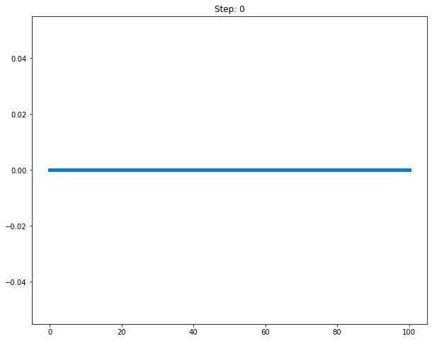
    plt.figure(figsize=(10, 4))
    plt.plot(line[:, 0], line[:, 1], linewidth=linewidth)
    plt.title("Step: 0")
    plt.axis("off")
    plt.show()

    steps_data = [segments]

    for step in range(steps):
        new_segments = []

        for segment in segments:
            result = sectional_formula(segment[:, 0], segment[:, 1])

            new_segments.append((result[0], result[1]))
            new_segments.append((result[2], result[3]))

        segments = np.array(new_segments)
        steps_data.append(segments)

        if show_all:
            plt.figure(figsize=(10, 4))

            for segment in segments:
                plt.plot(segment[:, 0], segment[:, 1], linewidth=linewidth)

            plt.title(f"Step: {step + 1}")
            plt.axis("off")
            plt.show()

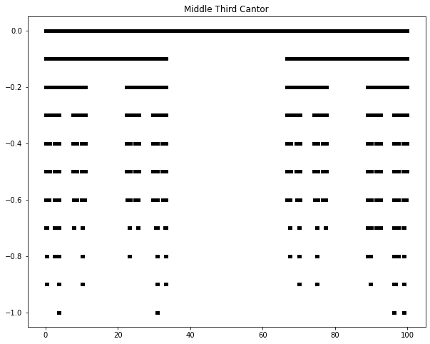
    plt.figure(figsize=(10, 8))

    for i, step_segments in enumerate(steps_data):
        for segment in step_segments:
            plt.plot(
                segment[:, 0],
                segment[:, 1] - 0.1 * i,
                linewidth=linewidth,
                color="black"
            )

    plt.title("Middle Third Cantor Set")
    plt.axis("off")
    plt.show()


middle_cantor()

Output:

Understanding the Cantor Set Code

The code starts with one line segment.

segments = [line]

At every step, each segment is divided into three parts.

result = sectional_formula(segment[:, 0], segment[:, 1])

Then we keep only the first and last parts.

new_segments.append((result[0], result[1]))
new_segments.append((result[2], result[3]))

The middle segment is removed.

After each iteration, the number of segments doubles.

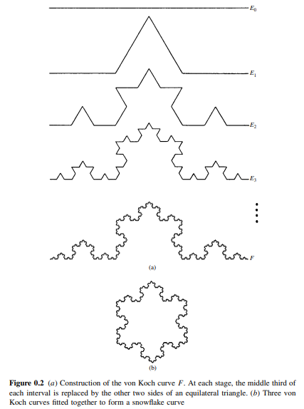
Von Koch Curve

The Von Koch Curve is another famous fractal. It is also known from the Koch snowflake construction.

The construction steps are:

1. Start with a straight line.
2. Divide the line into three equal parts.
3. Create an equilateral triangle on the middle part.
4. Remove the base of the triangle.
5. Treat every new segment as a line.
6. Repeat the same process.

FRACTAL GEOMETRY Mathematical Foundations and Applications: Page XIX

Koch Curve Idea

For each line segment, we replace it with four smaller segments.

The original line:

A ---------------- B

becomes:

A ---- C
       / \
      T
       \ /
D ---- B

The middle part becomes two sides of an equilateral triangle.

Von Koch Curve in Python

def von_koch(
    line=[(0, 0), (100, 0)],
    steps=5,
    linewidth=5,
    show_all=False,
    random_direction=True
):
    """Draw a Von Koch style curve."""
    line = np.array(line)
    segments = [line]

    plt.figure(figsize=(10, 4))
    plt.plot(line[:, 0], line[:, 1], linewidth=linewidth)
    plt.title("Step: 0")
    plt.axis("equal")
    plt.axis("off")
    plt.show()

    steps_data = [segments]

    for step in range(steps):
        new_segments = []

        for segment in segments:
            result = sectional_formula(segment[:, 0], segment[:, 1])

            (x1, y1) = result[0]
            (x3, y3) = result[1]
            (x4, y4) = result[2]
            (x2, y2) = result[3]

            if (x4 - x3) != 0:
                m1 = (y4 - y3) / (x4 - x3)

                m2 = (m1 - 3 ** 0.5) / (1 + 3 ** 0.5 * m1)
                m3 = (m1 + 3 ** 0.5) / (1 - 3 ** 0.5 * m1)

                if random_direction:
                    if int(np.random.random(1) * 1000) % 2 == 0:
                        m2, m3 = m3, m2

                xT = (y3 - y4 + m2 * x4 - m3 * x3) / (m2 - m3)
                yT = m2 * (xT - x4) + y4

                new_segments.append(((x1, y1), (x3, y3)))
                new_segments.append(((x3, y3), (xT, yT)))
                new_segments.append(((xT, yT), (x4, y4)))
                new_segments.append(((x4, y4), (x2, y2)))

        segments = np.array(new_segments)
        steps_data.append(segments)

        if show_all:
            plt.figure(figsize=(10, 8))

            for segment in segments:
                plt.plot(segment[:, 0], segment[:, 1], linewidth=linewidth)

            plt.title(f"Step: {step + 1}")
            plt.axis("equal")
            plt.axis("off")
            plt.show()

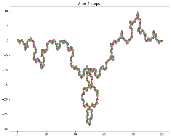
    plt.figure(figsize=(10, 8))

    for segment in segments:
        plt.plot(segment[:, 0], segment[:, 1], linewidth=linewidth)

    plt.title(f"After {steps} steps")
    plt.axis("equal")
    plt.axis("off")
    plt.show()


von_koch()

Output:

Explanation of the Koch Curve Code

The code follows these steps:

1. Prepare the first line segment.
2. Plot the initial line.
3. Loop through the number of steps.
4. For every current segment:
   • divide it into three parts
   • create an equilateral triangle from the middle part
   • remove the base
   • add four new segments
5. Plot the final result.

The most important part is finding the triangle point.

m1 = (y4 - y3) / (x4 - x3)

m2 = (m1 - 3 ** 0.5) / (1 + 3 ** 0.5 * m1)
m3 = (m1 + 3 ** 0.5) / (1 - 3 ** 0.5 * m1)

xT = (y3 - y4 + m2 * x4 - m3 * x3) / (m2 - m3)
yT = m2 * (xT - x4) + y4

Here:

• m1 is the slope of the middle segment
• m2 and m3 are slopes of the triangle sides
• (xT, yT) is the new triangle point

The slope formula comes from:

\[\tan(\theta) = \frac{m_1 - m_2}{1 + m_1 m_2}\]

For an equilateral triangle, the angle is 60 degrees.

A Cleaner Koch Curve Using Rotation Matrix

The previous code works, but we can make the Koch Curve easier using a rotation matrix.

To form an equilateral triangle, we rotate the middle segment by 60 degrees.

def rotate_point(point, angle_degrees):
    """Rotate a 2D point around the origin."""
    angle = np.radians(angle_degrees)

    rotation_matrix = np.array([
        [np.cos(angle), -np.sin(angle)],
        [np.sin(angle), np.cos(angle)]
    ])

    return rotation_matrix @ point

Now define a cleaner function.

def koch_curve_clean(line=[(0, 0), (100, 0)], steps=4):
    """Generate Koch curve points using vector rotation."""
    points = [np.array(line[0], dtype=float), np.array(line[1], dtype=float)]

    for _ in range(steps):
        new_points = []

        for i in range(len(points) - 1):
            p1 = points[i]
            p2 = points[i + 1]

            one_third = p1 + (p2 - p1) / 3
            two_third = p1 + 2 * (p2 - p1) / 3

            peak = one_third + rotate_point(two_third - one_third, 60)

            new_points.extend([p1, one_third, peak, two_third])

        new_points.append(points[-1])
        points = new_points

    points = np.array(points)

    plt.figure(figsize=(10, 6))
    plt.plot(points[:, 0], points[:, 1], color="black")
    plt.axis("equal")
    plt.axis("off")
    plt.title("Koch Curve")
    plt.show()


koch_curve_clean()

This version is shorter and easier to understand.

Sierpinski Triangle

The Sierpinski Triangle, also called the Sierpinski Gasket, is another famous fractal.

It can be created with these steps:

1. Start with a triangle.
2. Find the midpoint of each side.
3. Connect the midpoints to form a smaller upside-down triangle.
4. Remove the middle triangle.
5. Repeat the same process for the remaining three triangles.

A Python code of a modified version of the Sierpinski Gasket can be found in my GitHub repository:

• Fractal Geometry Repository

Sierpinski Triangle in Python

Here is a simple recursive version.

def midpoint(p1, p2):
    """Return midpoint of two points."""
    return ((p1[0] + p2[0]) / 2, (p1[1] + p2[1]) / 2)


def draw_triangle(points, color="black"):
    """Draw a triangle using three points."""
    triangle = plt.Polygon(points, fill=None, edgecolor=color)
    plt.gca().add_patch(triangle)


def sierpinski(points, depth):
    """Draw Sierpinski Triangle recursively."""
    if depth == 0:
        draw_triangle(points)
        return

    p1, p2, p3 = points

    m12 = midpoint(p1, p2)
    m23 = midpoint(p2, p3)
    m31 = midpoint(p3, p1)

    sierpinski([p1, m12, m31], depth - 1)
    sierpinski([m12, p2, m23], depth - 1)
    sierpinski([m31, m23, p3], depth - 1)


points = [(0, 0), (100, 0), (50, 86.6)]

plt.figure(figsize=(8, 8))
sierpinski(points, depth=5)
plt.axis("equal")
plt.axis("off")
plt.title("Sierpinski Triangle")
plt.show()

This recursive function keeps splitting triangles into smaller triangles.

Iteration vs Recursion in Fractals

Fractals can be generated using either iteration or recursion.

Iteration

Iteration uses loops.

Examples:

• Cantor Set
• Koch Curve implementation above

Recursion

Recursion means a function calls itself.

Examples:

• Sierpinski Triangle
• recursive tree fractals

Both approaches work. Recursion often matches the mathematical definition of fractals more naturally, but iteration can sometimes be easier to control.

Practical Tips for Drawing Fractals

Here are a few tips:

• Start with a small number of steps.
• Increase steps slowly.
• Use plt.axis("equal") to avoid distortion.
• Use thin lines for deeper fractals.
• Avoid too many iterations because the number of segments grows quickly.
• Save figures with high resolution if needed.

Example:

plt.savefig("fractal.png", dpi=300, bbox_inches="tight")

Complexity of Fractals

Fractals grow quickly with each step.

For the Cantor Set:

number of segments = 2^steps

For the Koch Curve:

number of segments = 4^steps

This means that increasing from 5 steps to 10 steps can greatly increase computation and plotting time.

Exercises

Try these exercises:

1. Change the number of steps in the Cantor Set.
2. Change the starting line length.
3. Draw the Koch Curve without random direction.
4. Create a Koch snowflake by starting with a triangle.
5. Change the color of fractal lines.
6. Save the fractal output as a PNG file.
7. Create a Sierpinski Triangle with different depths.
8. Try drawing a fractal tree with recursion.

Final Thoughts

In this post, we created fractal shapes with Python using NumPy and Matplotlib. We started with the Middle Third Cantor Set, then created the Von Koch Curve, and finally added a simple Sierpinski Triangle example.

Fractals are beautiful because simple rules can create complex patterns. Python makes it easy to experiment with those rules and visualize the results.

This is only the beginning. You can extend these ideas to draw Koch snowflakes, fractal trees, Mandelbrot sets, Julia sets, and many other mathematical patterns.