Stock Backtesting in Python: Beginner Guide with Backtesting.py, yfinance, SMA, EMA, and PPO

13 minute read

Stock backtesting in Python is a way to test a trading idea on historical market data. Instead of risking real money directly, we first ask a simple question:

If I had followed this strategy in the past, what would have happened?

Backtesting does not guarantee future profit. A strategy that worked well in the past can still fail in the future. But backtesting is useful because it helps us understand how a strategy behaves, how often it trades, how much drawdown it has, and whether the idea is worth studying further.

In this post, I will explain the basics of stock backtesting using Python. We will start with a simple moving average crossover idea, first manually with pandas and then using the popular Backtesting.py package.

We will cover:

what stock backtesting means
how to download stock data with yfinance
how to calculate simple moving averages
how to create a simple SMA crossover strategy
how to backtest the same strategy with Backtesting.py
how to use take profit and stop loss
how to test EMA crossover and PPO strategies
why backtesting results should be treated carefully

This post is for learning and educational purposes only. It is not financial advice.

A Simple Story About Backtesting

Imagine two friends, John and Joe. They both earned some money from their jobs and wanted to invest in the stock market.

Joe followed the market trend. He bought a stock because he saw the price going up. After a few days, the stock price increased, and he felt happy.

John was calmer. He knew that a position increasing in value does not mean real profit until the stock is sold. He asked a different question:

What if I had bought this stock whenever my strategy gave a buy signal and sold it whenever my strategy gave a sell signal? How much money would I have today?

That question is the beginning of backtesting.

In this blog, we will use a simple strategy:

buy when a short moving average crosses above a long moving average
sell when the short moving average crosses below the long moving average

This is not a perfect strategy. It is only a simple example to learn the workflow.

What Is Stock Backtesting?

Stock backtesting means testing a trading strategy using historical price data.

A backtest usually needs:

historical price data
a trading rule
starting cash
position sizing logic
entry rules
exit rules
trading costs or commission
performance metrics

For example, a simple trading rule can be:

Buy when SMA 20 crosses above SMA 40.
Sell when SMA 20 crosses below SMA 40.

Backtesting helps us answer questions such as:

How much return did the strategy make?
How many trades did it take?
What was the maximum drawdown?
How many trades were profitable?
Did the strategy beat buy and hold?
Did commissions reduce profit?
Was the strategy too risky?

Install Required Python Packages

We will use backtesting, yfinance, pandas, and later pandas_ta.

pip install backtesting yfinance pandas pandas-ta

In a notebook, you can run:

!pip install backtesting
!pip install yfinance
!pip install pandas-ta

I removed the long installation output from this post because it is not useful for readers.

Import Python Packages

import pandas as pd
import yfinance as yf

We will use:

pandas for data handling
yfinance for downloading stock price data
Backtesting.py for strategy testing

Download Stock Data with yfinance

For this tutorial, we will use Apple stock data.

data = yf.download("AAPL", start="2015-01-01", end="2022-04-30")

data = data.drop(columns=["Adj Close", "Volume"])
data.head()

The data contains four important columns:

Open
High
Low
Close

For Backtesting.py, the column names should follow the OHLC format:

Open
High
Low
Close
Volume if available

In this example, I removed Adj Close and Volume to keep the tutorial simple.

Using Built-in Sample Data from Backtesting.py

Backtesting.py also provides sample data. For example:

import backtesting.test as btest

btest.GOOG.head()

This gives sample Google price data. But in this post, we will mainly use AAPL data downloaded from yfinance.

What Is a Simple Moving Average?

A Simple Moving Average, or SMA, is the average price over a fixed number of previous periods.

For example:

SMA 20 means the average closing price of the last 20 trading days
SMA 40 means the average closing price of the last 40 trading days

A moving average helps smooth noisy price movement.

A common trading idea is:

when the short SMA goes above the long SMA, momentum may be positive
when the short SMA goes below the long SMA, momentum may be negative

This is called a moving average crossover strategy.

Calculate SMA in pandas

Let’s calculate SMA 20 and SMA 40.

n1, n2 = 20, 40

ndata = data.copy()

ndata[f"SMA_{n1}"] = ndata["Close"].rolling(n1).mean()
ndata[f"SMA_{n2}"] = ndata["Close"].rolling(n2).mean()

ndata[[f"SMA_{n1}", f"SMA_{n2}"]].plot(figsize=(15, 10))

png

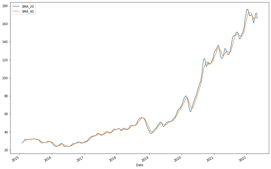
The two moving averages cross each other multiple times. These crossover points can be used as possible buy and sell signals.

Plot Only the Last 200 Days

The full chart can look too large, so let’s look at only the last 200 days.

last = 200
n1, n2 = 20, 40

tdata = data.copy().tail(last)

tdata[f"SMA_{n1}"] = tdata["Close"].rolling(n1).mean()
tdata[f"SMA_{n2}"] = tdata["Close"].rolling(n2).mean()

tdata[[f"SMA_{n1}", f"SMA_{n2}"]].plot(figsize=(15, 10))

png

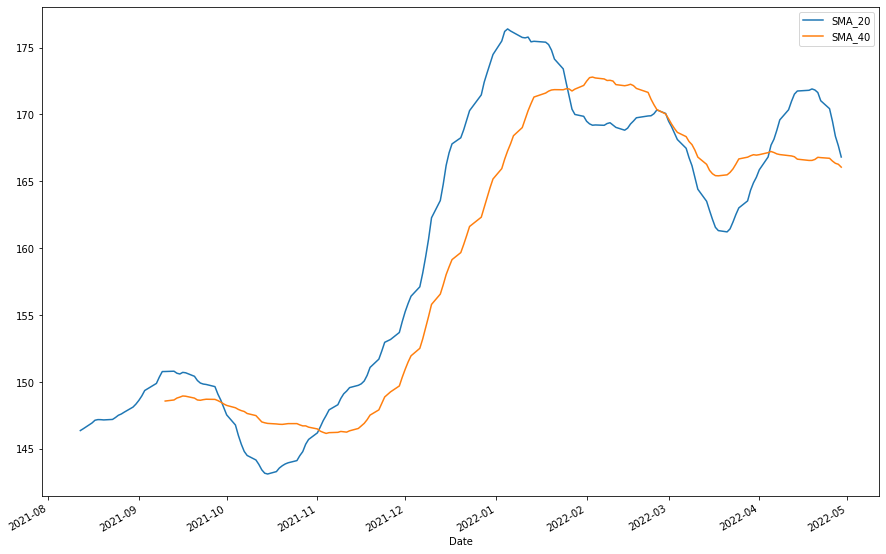
Now the crossover points are easier to see.

Define a Simple SMA Crossover Strategy

The strategy is:

Buy when SMA 20 crosses above SMA 40.
Sell when SMA 20 crosses below SMA 40.
Use the next day’s open price for trade execution.
Start with $10,000.
Buy as many shares as possible.
Sell all shares when the sell signal appears.

This is a very simple strategy. It does not include taxes, slippage, spread, or realistic order execution.

Find SMA Crossover Points

First, we check whether SMA 20 is greater than SMA 40.

tdata["sma1_gt_sma2"] = tdata[f"SMA_{n1}"] > tdata[f"SMA_{n2}"]

Then we check when this condition changes.

tdata["crossed"] = tdata["sma1_gt_sma2"] != tdata["sma1_gt_sma2"].shift(1)

print(f"Number of crosses: {tdata['crossed'].sum() - 1}")

The first cross is ignored because it comes from the shifted missing value.

Manual Backtesting Logic

Now, let’s manually backtest this crossover strategy.

ntdata = tdata.reset_index().copy()

# Use yesterday's signal to trade at today's open
ntdata["crossed"] = ntdata["crossed"].shift(1)
ntdata["sma1_gt_sma2"] = ntdata["sma1_gt_sma2"].shift(1)

positions = 0
remaining_amount = 10000
last_row = len(ntdata) - 1

trades = []
trade_info = []

for i, row in ntdata.iterrows():
    if i != 0:
        # Buy signal
        if row.crossed and row.sma1_gt_sma2:
            positions = int(remaining_amount / row.Open)
            remaining_amount = remaining_amount - row.Open * positions

            trade_info.append(positions)
            trade_info.append(row.Open)
            trade_info.append(row.Date)

        # Sell signal
        if row.crossed and row.sma1_gt_sma2 == False and positions > 0:
            remaining_amount = remaining_amount + row.Open * positions

            trade_info.append(row.Date)
            trade_info.append(row.Open)

            trades.append(trade_info)

            trade_info = []
            positions = 0

    # Sell remaining position on last day
    if i == last_row and positions > 0:
        remaining_amount = remaining_amount + positions * row.Open

        trade_info.append(row.Date)
        trade_info.append(row.Open)

        trades.append(trade_info)

        positions = 0

trades = pd.DataFrame(
    trades,
    columns=["Positions", "Buy", "Entry", "Exit", "Sell"]
)

trades["return"] = ((trades["Sell"] - trades["Buy"]) * trades["Positions"]).cumsum()

trades

In the last 200 days, this strategy ended with an overall loss of around $457.

This is a useful lesson: a strategy can look reasonable but still lose money over a particular period.

Test the Same Strategy on a Larger Period

Now let’s test the same strategy on the last 1000 trading days.

n1, n2 = 20, 40
last = 1000

tdata = data.copy().tail(last)

tdata[f"SMA_{n1}"] = tdata["Close"].rolling(n1).mean()
tdata[f"SMA_{n2}"] = tdata["Close"].rolling(n2).mean()

tdata["sma1_gt_sma2"] = tdata[f"SMA_{n1}"] > tdata[f"SMA_{n2}"]
tdata["crossed"] = tdata["sma1_gt_sma2"] != tdata["sma1_gt_sma2"].shift(1)

print(f"Number of crosses: {tdata['crossed'].sum() - 1}")

Using the larger period, the strategy made money in this AAPL example.

This is another important lesson: backtest results depend heavily on the selected time period. A strategy can lose money in one period and make money in another.

Manual Backtesting vs Backtesting.py

Until now, we wrote our own backtesting logic. This is useful for learning, but it becomes difficult when we want to handle:

multiple trades
commissions
short selling
stop loss
take profit
position sizing
equity curve
drawdown
performance metrics
strategy plots

That is why packages like Backtesting.py are useful.

SMA Crossover Strategy with Backtesting.py

The following strategy is modified from the Backtesting.py quick start example.

from backtesting import Strategy
from backtesting.lib import crossover
from backtesting.test import SMA


class SmaCross(Strategy):
    # Moving average periods
    n1 = 20
    n2 = 40

    def init(self):
        # Precompute moving averages
        self.sma1 = self.I(SMA, self.data.Close, self.n1)
        self.sma2 = self.I(SMA, self.data.Close, self.n2)

    def next(self):
        # Buy when SMA 20 crosses above SMA 40
        if crossover(self.sma1, self.sma2):
            self.position.close()
            self.buy()

        # Sell when SMA 40 crosses above SMA 20
        elif crossover(self.sma2, self.sma1):
            self.position.close()
            self.sell()

Now run the backtest.

from backtesting import Backtest

bt = Backtest(
    data.tail(last),
    SmaCross,
    cash=10000,
    commission=0
)

stats = bt.run()
stats

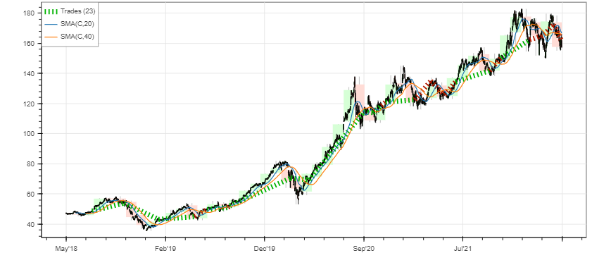
The backtest result from the original experiment was:

Metric	Value
Final Equity	`$21,836.20`
Return	`118.36%`
Buy & Hold Return	`234.38%`
Max Drawdown	`-38.69%`
Number of Trades	`23`
Win Rate	`52.17%`
Profit Factor	`2.83`

The strategy made money, but it did not beat buy and hold in this AAPL period.

That is important. A profitable strategy is not always a good strategy if simply holding the stock would have performed better.

Understanding Backtesting.py Metrics

Backtesting.py returns many metrics. Some important ones are:

Equity Final

The final account value after all trades.

Return

The percentage gain or loss from the starting cash.

Buy & Hold Return

The return from simply buying the stock at the beginning and holding it until the end.

Exposure Time

The percentage of time the strategy had an open position.

Max Drawdown

The largest percentage drop from an equity peak to a later low.

Win Rate

The percentage of trades that were profitable.

Profit Factor

Gross profit divided by gross loss. A value above 1 means total profit is greater than total loss.

Sharpe Ratio

A risk-adjusted return metric. Higher is generally better, but it should not be the only metric used.

View Individual Trades

The trade table can be accessed from the stats object.

stats["_trades"]

This table contains information such as:

trade size
entry price
exit price
profit and loss
return percentage
entry date
exit date
trade duration

This is useful for analyzing how each trade performed.

Plot the Backtest Result

Backtesting.py can generate an interactive Bokeh plot.

bt.plot()

png png png

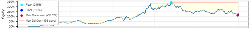
These plots help us inspect trades, equity curve, drawdown, and price movement.

Add Take Profit and Stop Loss

Take profit and stop loss are used to exit trades automatically.

Take profit exits when the trade reaches a target profit.
Stop loss exits when the trade reaches a maximum allowed loss.

In this example:

take profit is set at 20% above the current close price
stop loss is set at 5% below the current close price

from backtesting import Strategy
from backtesting.lib import crossover
from backtesting.test import SMA


class SmaCrossWithTPSL(Strategy):
    n1 = 20
    n2 = 40

    def init(self):
        self.sma1 = self.I(SMA, self.data.Close, self.n1)
        self.sma2 = self.I(SMA, self.data.Close, self.n2)

    def next(self):
        if crossover(self.sma1, self.sma2):
            self.buy(
                tp=self.data.Close[-1] * 1.20,
                sl=self.data.Close[-1] * 0.95
            )

        elif crossover(self.sma2, self.sma1):
            self.position.close()

Run the backtest:

bt = Backtest(
    data.tail(last),
    SmaCrossWithTPSL,
    cash=10000,
    commission=0
)

stats = bt.run()
stats

The original result was:

Metric	Value
Final Equity	`$25,715.43`
Return	`157.15%`
Buy & Hold Return	`234.38%`
Max Drawdown	`-10.93%`
Number of Trades	`12`
Win Rate	`66.67%`
Profit Factor	`8.89`

The strategy improved compared to the previous SMA strategy, especially in drawdown. But it still did not beat buy and hold in that period.

EMA Crossover Strategy

Now let’s try another strategy using Exponential Moving Averages, or EMA.

An EMA gives more weight to recent prices. This makes it react faster than SMA.

The strategy idea is:

Buy if EMA 9 crosses above EMA 20.
Also buy if EMA 50 crosses above EMA 100.
Close positions if EMA 9 crosses below EMA 20.
Also close positions if EMA 50 crosses below EMA 100.

We can calculate EMA using pandas_ta.

import pandas_ta as ta

from backtesting import Backtest
from backtesting import Strategy
from backtesting.lib import crossover


class EmaCross(Strategy):
    def init(self):
        self.ema9 = self.I(ta.ema, pd.Series(self.data.Close), 9)
        self.ema20 = self.I(ta.ema, pd.Series(self.data.Close), 20)
        self.ema50 = self.I(ta.ema, pd.Series(self.data.Close), 50)
        self.ema100 = self.I(ta.ema, pd.Series(self.data.Close), 100)

    def next(self):
        if crossover(self.ema9, self.ema20) or crossover(self.ema50, self.ema100):
            self.buy()

        elif crossover(self.ema20, self.ema9) or crossover(self.ema100, self.ema50):
            self.position.close()

Run the strategy:

bt = Backtest(
    data,
    EmaCross,
    cash=10000,
    commission=0.02
)

stats = bt.run()
bt.plot()

stats

png png png

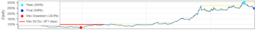
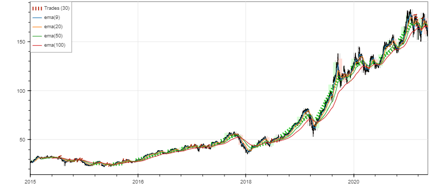
The original result was:

Metric	Value
Final Equity	`$24,777.30`
Return	`147.77%`
Buy & Hold Return	`476.79%`
Max Drawdown	`-28.46%`
Number of Trades	`30`
Win Rate	`46.67%`
Profit Factor	`2.58`

This strategy made money, but it performed much worse than buy and hold for AAPL over the full period.

This is why we should always compare a strategy with a simple benchmark.

Percentage Price Oscillator Strategy

The Percentage Price Oscillator, or PPO, is a momentum indicator.

It is similar to MACD, but it expresses the difference between moving averages as a percentage.

The PPO usually contains:

PPO line
signal line
histogram

A common idea is:

buy when the PPO line crosses above the signal line
sell or close when the PPO line crosses below the signal line

I explained technical indicators in another blog:

Python for Stock Market Analysis: Technical Indicators

pandas_ta already provides PPO, so we do not need to write it from scratch.

ta.ppo(data.Close)

Now create the PPO strategy.

class PPO(Strategy):
    def init(self):
        self.ppo = self.I(ta.ppo, pd.Series(self.data.Close))

    def next(self):
        # PPO line crosses above signal line
        if crossover(self.ppo[0], self.ppo[2]):
            self.buy()

        # Signal line crosses above PPO line
        elif crossover(self.ppo[2], self.ppo[0]):
            self.position.close()

Run the strategy on AAPL.

bt = Backtest(
    data,
    PPO,
    cash=10000,
    commission=0.02
)

stats = bt.run()
bt.plot()

print(stats)

png png png png

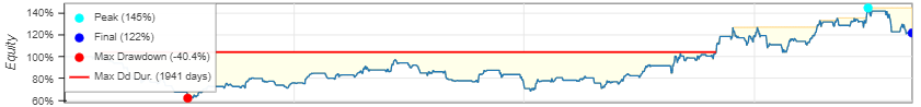
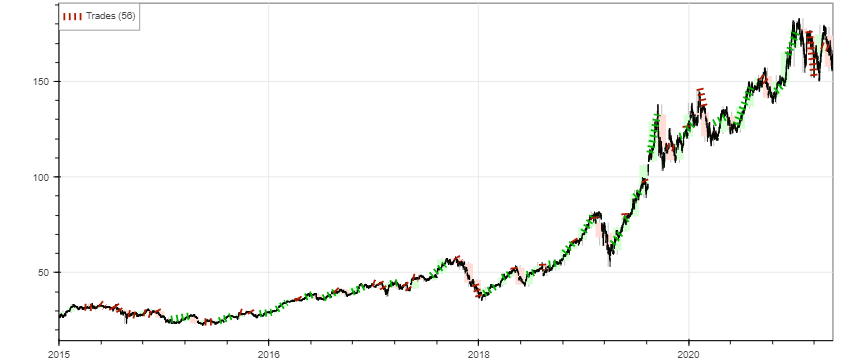
The original AAPL PPO result was:

Metric	Value
Final Equity	`$12,163.35`
Return	`21.63%`
Buy & Hold Return	`476.79%`
Max Drawdown	`-40.43%`
Number of Trades	`56`
Win Rate	`44.64%`
Profit Factor	`1.24`

This strategy made a small profit, but it performed very poorly compared to buy and hold.

Test PPO on BABA

A strategy that makes money on one stock can fail badly on another stock. To test this, let’s run PPO on BABA.

bdata = yf.download("BABA", start="2015-01-01", end="2022-11-30")

bdata = bdata.drop(columns=["Adj Close", "Volume"])

bt = Backtest(
    bdata,
    PPO,
    cash=10000,
    commission=0.02
)

stats = bt.run()
bt.plot()

print(stats)

png png png png

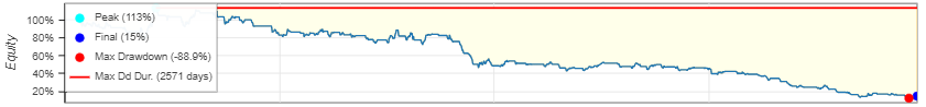
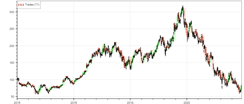
The original BABA PPO result was:

Metric	Value
Final Equity	`$1,485.46`
Return	`-85.15%`
Buy & Hold Return	`-22.32%`
Max Drawdown	`-88.92%`
Number of Trades	`71`
Win Rate	`26.76%`
Profit Factor	`0.50`

This is a very bad result. It shows that a strategy that looks acceptable on AAPL can completely fail on BABA.

Lessons from These Backtests

The examples above show some important lessons.

A Profitable Strategy Is Not Always a Good Strategy

The strategy may make money but still underperform buy and hold.

Time Period Matters

A strategy may perform well in one period and fail in another.

One Stock Is Not Enough

Testing only on one stock can be misleading.

Commissions Matter

Even small commissions can reduce returns, especially for strategies that trade often.

Drawdown Is Important

A strategy with high return but huge drawdown may be hard to follow in real life.

Overfitting Is Dangerous

If you keep changing parameters until the backtest looks good, the strategy may only be fitted to the past.

Common Backtesting Mistakes

Here are common mistakes beginners should avoid:

using future data accidentally
ignoring trading fees
ignoring slippage
testing on only one stock
testing on only one time period
optimizing too many parameters
not comparing with buy and hold
ignoring drawdown
assuming backtest profit means future profit
using unrealistic position sizing
forgetting that real market orders may not fill at the expected price

Backtesting is useful, but it is not magic.

Simple Checklist Before Trusting a Backtest

Before trusting a strategy, ask:

Did I include commission?
Did I avoid future leakage?
Did I compare with buy and hold?
Did I test multiple stocks?
Did I test different time periods?
Did I check max drawdown?
Did I inspect individual trades?
Did I avoid over-optimizing parameters?
Is the strategy logic simple and explainable?
Would I still follow it during a losing period?

If the answer is no to many of these questions, the strategy needs more testing.

Final Thoughts

In this post, we learned the basics of stock backtesting in Python. We started with a manual SMA crossover backtest using pandas, then used Backtesting.py to test SMA, EMA, and PPO strategies.

The main lesson is that backtesting helps us study trading ideas, but it does not guarantee profit. Some strategies may look good on one stock and fail on another. Some may make money but still lose against buy and hold.

A good next step would be to test more strategies, add realistic costs, compare multiple assets, and evaluate risk more carefully.

There are many features in Backtesting.py, and I will cover more advanced backtesting ideas in the next part.

Twitter Facebook LinkedIn

Quassarian Viper